This is part 1 in a 3-part series about the Second Law:

The Mystery of the Second Law
Entropy increases. Mechanical work irreversibly turns into heat. The Second Law of thermodynamics is considered one of the great general principles of physical science. But 150 years after it was first introduced, there’s still something deeply mysterious about the Second Law. It almost seems like it’s going to be “provably true”. But one never quite gets there; it always seems to need something extra. Sometimes textbooks will gloss over everything; sometimes they’ll give some kind of “common-sense-but-outside-of-physics argument”. But the mystery of the Second Law has never gone away.
Why does the Second Law work? And does it even in fact always work, or is it actually sometimes violated? What does it really depend on? What would be needed to “prove it”?
For me personally the quest to understand the Second Law has been no less than a 50-year story. But back in the 1980s, as I began to explore the computational universe of simple programs, I discovered a fundamental phenomenon that was immediately reminiscent of the Second Law. And in the 1990s I started to map out just how this phenomenon might finally be able to demystify the Second Law. But it is only now—with ideas that have emerged from our Physics Project—that I think I can pull all the pieces together and finally be able to construct a proper framework to explain why—and to what extent—the Second Law is true.
In its usual conception, the Second Law is a law of thermodynamics, concerned with the dynamics of heat. But it turns out that there’s a vast generalization of it that’s possible. And in fact my key realization is that the Second Law is ultimately just a manifestation of the very same core computational phenomenon that is at the heart of our Physics Project and indeed the whole conception of science that is emerging from our study of the ruliad and the multicomputational paradigm.
It’s all a story of the interplay between underlying computational irreducibility and our nature as computationally bounded observers. Other observers—or even our own future technology—might see things differently. But at least for us now the ubiquity of computational irreducibility leads inexorably to the generation of behavior that we—with our computationally bounded nature—will read as “random”. We might start from something highly ordered (like gas molecules all in the corner of a box) but soon—at least as far as we’re concerned—it will typically seem to “randomize”, just as the Second Law implies.
In the twentieth century there emerged three great physical theories: general relativity, quantum mechanics and statistical mechanics, with the Second Law being the defining phenomenon of statistical mechanics. But while there was a sense that statistical mechanics (and in particular the Second Law) should somehow be “formally derivable”, general relativity and quantum mechanics seemed quite different. But our Physics Project has changed that picture. And the remarkable thing is that it now seems as if all three of general relativity, quantum mechanics and statistical mechanics are actually derivable, and from the same ultimate foundation: the interplay between computational irreducibility and the computational boundedness of observers like us.
The case of statistical mechanics and the Second Law is in some ways simpler than the other two because in statistical mechanics it’s realistic to separate the observer from the system they’re observing, while in general relativity and quantum mechanics it’s essential that the observer be an integral part of the system. It also helps that phenomena about things like molecules in statistical mechanics are much more familiar to us today than those about atoms of space or branches of multiway systems. And by studying the Second Law we’ll be able to develop intuition that we can use elsewhere, say in discussing “molecular” vs. “fluid” levels of description in my recent exploration of the physicalization of the foundations of metamathematics.
The Core Phenomenon of the Second Law
The earliest statements of the Second Law were things like: “Heat doesn’t flow from a colder body to a hotter one” or “You can’t systematically purely convert heat to mechanical work”. Later on there came the somewhat more abstract statement “Entropy tends to increase”. But in the end, all these statements boil down to the same idea: that somehow things always tend to get progressively “more random”. What may start in an orderly state will—according to the Second Law—inexorably “degrade” to a “randomized” state.
But how general is this phenomenon? Does it just apply to heat and temperature and molecules and things? Or is it something that applies across a whole range of kinds of systems?
The answer, I believe, is that underneath the Second Law there’s a very general phenomenon that’s extremely robust. And that has the potential to apply to pretty much any kind of system one can imagine.
Here’s a longtime favorite example of mine: the rule 30 cellular automaton:

Start from a simple “orderly” state, here containing just a single non-white cell. Then apply the rule over and over again. The pattern that emerges has some definite, visible structure. But many aspects of it “seem random”. Just as in the Second Law, even starting from something “orderly”, one ends up getting something “random”.
But is it “really random”? It’s completely determined by the initial condition and rule, and you can always recompute it. But the subtle yet critical point is that if you’re just given the output, it can still “seem random” in the sense that no known methods operating purely on this output can find regularities in it.
It’s reminiscent of the situation with something like the digits of π. There’s a fairly simple algorithm for generating these digits. Yet once generated, the digits on their own seem for practical purposes random.
In studying physical systems there’s a long history of assuming that whenever randomness is seen, it somehow comes from outside the system. Maybe it’s the effect of “thermal noise” or “perturbations” acting on the system. Maybe it’s chaos-theory-style “excavation” of higher-order digits supplied through real-number initial conditions. But the surprising discovery I made in the 1980s by looking at things like rule 30 is that actually no such “external source” is needed: instead, it’s perfectly possible for randomness to be generated intrinsically within a system just through the process of applying definite underlying rules.
How can one understand this? The key is to think in computational terms. And ultimately the source of the phenomenon is the interplay between the computational process associated with the actual evolution of the system and the computational processes that our perception of the output of that evolution brings to bear.
We might have thought if a system had a simple underlying rule—like rule 30—then it’d always be straightforward to predict what the system will do. Of course, we could in principle always just run the rule and see what happens. But the question is whether we can expect to “jump ahead” and “find the outcome”, with much less computational effort than the actual evolution of the system involves.
And an important conclusion of a lot of science I did in the 1980s and 1990s is that for many systems—presumably including rule 30—it’s simply not possible to “jump ahead”. And instead the evolution of the system is what I call computationally irreducible—so that it takes an irreducible amount of computational effort to find out what the system does.
Ultimately this is a consequence of what I call the Principle of Computational Equivalence, which states that above some low threshold, systems always end up being equivalent in the sophistication of the computations they perform. And this is why even our brains and our most sophisticated methods of scientific analysis can’t “computationally outrun” even something like rule 30, so that we must consider it computationally irreducible.
So how does this relate to the Second Law? It’s what makes it possible for a system like rule 30 to operate according to a simple underlying rule, yet to intrinsically generate what seems like random behavior. If we could do all the necessary computationally irreducible work then we could in principle “see through” to the simple rules underneath. But the key point (emphasized by our Physics Project) is that observers like us are computationally bounded in our capabilities. And this means that we’re not able to “see through the computational irreducibility”—with the result that the behavior we see “looks random to us”.
And in thermodynamics that “random-looking” behavior is what we associate with heat. And the Second Law assertion that energy associated with systematic mechanical work tends to “degrade into heat” then corresponds to the fact that when there’s computational irreducibility the behavior that’s generated is something we can’t readily “computationally see through”—so that it appears random to us.
The Road from Ordinary Thermodynamics
Systems like rule 30 make the phenomenon of intrinsic randomness generation particularly clear. But how do such systems relate to the ones that thermodynamics usually studies? The original formulation of the Second Law involved gases, and the vast majority of its applications even today still concern things like gases.
At a basic level, a typical gas consists of a collection of discrete molecules that interact through collisions. And as an idealization of this, we can consider hard spheres that move according to the standard laws of mechanics and undergo perfectly elastic collisions with each other, and with the walls of a container. Here’s an example of a sequence of snapshots from a simulation of such a system, done in 2D:

We begin with an organized “flotilla” of “molecules”, systematically going in a particular direction (and not touching, to avoid a “Newton’s cradle” many-collisions-at-a-time effect). But after these molecules collide with a wall, they quickly start to move in what seem like much more random ways. The original systematic motion is like what happens when one is “doing mechanical work”, say moving a solid object. But what we see is that—just as the Second Law implies—this motion is quickly “degraded” into disordered and seemingly random “heat-like” microscopic motion.
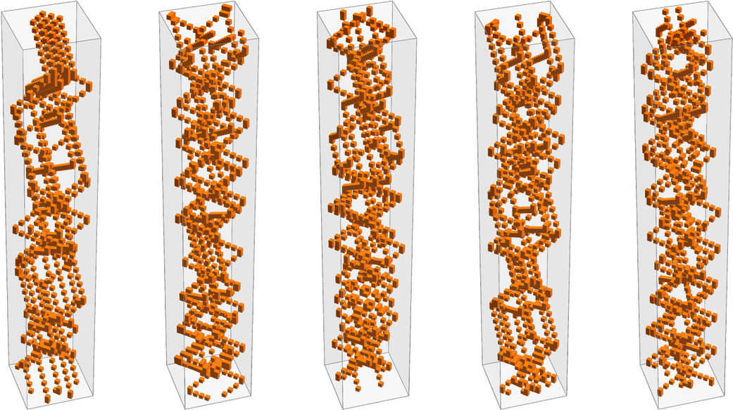
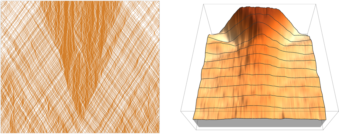
Here’s a “spacetime” view of the behavior:

Looking from far away, with each molecule’s spacetime trajectory shown as a slightly transparent tube, we get:

There’s already some qualitative similarity with the rule 30 behavior we saw above. But there are many detailed differences. And one of the most obvious is that while rule 30 just has a discrete collection of cells, the spheres in the hard-sphere gas can be at any position. And, what’s more, the precise details of their positions can have an increasingly large effect. If two elastic spheres collide perfectly head-on, they’ll bounce back the way they came. But as soon as they’re even slightly off center they’ll bounce back at a different angle, and if they do this repeatedly even the tiniest initial off-centeredness will be arbitrarily amplified:

And, yes, this chaos-theory-like phenomenon makes it very difficult even to do an accurate simulation on a computer with limited numerical precision. But does it actually matter to the core phenomenon of randomization that’s central to the Second Law?
To begin testing this, let’s consider not hard spheres but instead hard squares (where we assume that the squares always stay in the same orientation, and ignore the mechanical torques that would lead to spinning). If we set up the same kind of “flotilla” as before, with the edges of the squares aligned with the walls of the box, then things are symmetrical enough that we don’t see any randomization—and in fact the only nontrivial thing that happens is a little

Viewed in “spacetime” we can see the “flotilla” is just bouncing unchanged off the walls:

But remove even a tiny bit of the symmetry—here by roughly doubling the “masses” of some of the squares and “riffling” their positions (which also avoids singular multi-square collisions)—and we get:

In “spacetime” this becomes

or “from the side”:

So despite the lack of chaos-theory-like amplification behavior (or any associated loss of numerical precision in our simulations), there’s still rapid “degradation” to a certain apparent randomness.
So how much further can we go? In the hard-square gas, the squares can still be at any location, and be moving at any speed in any direction. As a simpler system (that I happened to first investigate a version of nearly 50 years ago), let’s consider a discrete grid in which idealized molecules have discrete directions and are either present or not on each edge:

The system operates in discrete steps, with the molecules at each step moving or “scattering” according to the rules (up to rotations)

and interacting with the “walls” according to:

Running this starting with a “flotilla” we get on successive steps:

Or, sampling every 10 steps:

In “spacetime” this becomes (with the arrows tipped to trace out “worldlines”)

or “from the side”:

And again we see at least a certain level of “randomization”. With this model we’re getting quite close to the setup of something like rule 30. And reformulating this same model we can get even closer. Instead of having “particles” with explicit “velocity directions”, consider just having a grid in which an alternating pattern of 2×2 blocks are updated at each step according to

and the “wall” rules
as well as the “rotations” of all these rules. With this “block cellular automaton” setup, “isolated particles” move according to the ![]() rule like the pieces on a checkerboard:
rule like the pieces on a checkerboard:

A “flotilla” of particles—like equal-mass hard squares—has rather simple behavior in the “square enclosure”:

In “spacetime” this is just:

But if we add even a single fixed (“single-cell-of-wall”) “obstruction cell” (here at the very center of the box, so preserving reflection symmetry) the behavior is quite different:

In “spacetime” this becomes (with the “obstruction cell” shown in gray)

or “from the side” (with the “obstruction” sometimes getting obscured by cells in front):

As it turns out, the block cellular automaton model we’re using here is actually functionally identical to the “discrete velocity molecules” model we used above, as the correspondence of their rules indicates:

And seeing this correspondence one gets the idea of considering a “rotated container”—which no longer gives simple behavior even without any kind of “interior fixed obstruction cell”:

Here’s the corresponding “spacetime” view
and here’s what it looks like “from the side”:

Here’s a larger version of the same setup (though no longer with exact symmetry) sampled every 50 steps:

And, yes, it’s increasingly looking as if there’s intrinsic randomness generation going on, much like in rule 30. But if we go a little further the correspondence becomes even clearer.
The systems we’ve been looking at so far have all been in 2D. But what if—like in rule 30—we consider 1D? It turns out we can set up very much the same kind of “gas-like” block cellular automata. Though with blocks of size 2 and two possible values for each cell, there’s only one viable rule
where in effect the only nontrivial transformation is:
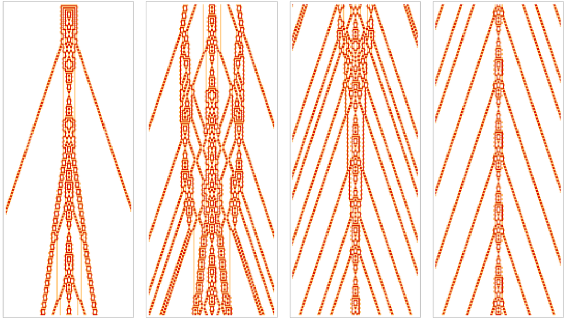
(In 1D we can also make things simpler by not using explicit “walls”, but instead just wrapping the array of cells around cyclically.) Here’s then what happens with this rule with a few possible initial states:

And what we see is that in all cases the “particles” effectively just “pass through each other” without really “interacting”. But we can make there be something closer to “real interactions” by introducing another color, and adding a transformation which effectively introduces a “time delay” to each “crossover” of particles (as an alternative, one can also stay with 2 colors, and use size-3 blocks):
And with this “delayed particle” rule (that, as it happens, I first studied in 1986) we get:

With sufficiently simple initial conditions this still gives simple behavior, such as:

But as soon as one reaches the 121st initial condition (![]() ) one sees:
) one sees:

(As we’ll discuss below, in a finite-size region of the kind we’re using, it’s inevitable that the pattern eventually repeats, though in the particular case shown it takes 7022 steps.) Here’s a slightly larger example, in which there’s clearer “progressive degradation” of the initial condition to apparent randomness:

We’ve come quite far from our original hard-sphere “realistic gas molecules”. But there’s even further to go. With hard spheres there’s built-in conservation of energy, momentum and number of particles. And we don’t specifically have these things anymore. But the rule we’re using still does have conservation of the number of non-white cells. Dropping this requirement, we can have rules like
which gradually “fill in with particles”:

What happens if we just let this “expand into a vacuum”, without any “walls”? The behavior is complex. And as is typical when there’s computational irreducibility, it’s at first hard to know what will happen in the end. For this particular initial condition everything becomes essentially periodic (with period 70) after 979 steps:
But with a slightly different initial condition, it seems to have a good chance of growing forever:

With slightly different rules (that here happen not be left-right symmetric) we start seeing rapid “expansion into the vacuum”—basically just like rule 30:

The whole setup here is very close to what it is for rule 30. But there’s one more feature we’ve carried over here from our hard-sphere gas and other models. Just like in standard classical mechanics, every part of the underlying rule is reversible, in the sense that if the rule says that block u goes to block v it also says that block v goes to block u.
Rules like

remove this restriction but produce behavior that’s qualitatively no different from the reversible rules above.
But now we’ve got to systems that are basically set up just like rule 30. (They happen to be block cellular automata rather than ordinary ones, but that really doesn’t matter.) And, needless to say, being set up like rule 30 it shows the same kind of intrinsic randomness generation that we see in a system like rule 30.
We started here from a “physically realistic” hard-sphere gas model—which we’ve kept on simplifying and idealizing. And what we’ve found is that through all this simplification and idealization, the same core phenomenon has remained: that even starting from “simple” or “ordered” initial conditions, complex and “apparently random” behavior is somehow generated, just like it is in typical Second Law behavior.
At the outset we might have assumed that to get this kind of “Second Law behavior” would need at least quite a few features of physics. But what we’ve discovered is that this isn’t the case. And instead we’ve got evidence that the core phenomenon is much more robust and in a sense purely computational.
Indeed, it seems that as soon as there’s computational irreducibility in a system, it’s basically inevitable that we’ll see the phenomenon. And since from the Principle of Computational Equivalence we expect that computational irreducibility is ubiquitous, the core phenomenon of the Second Law will in the end be ubiquitous across a vast range of systems, from things like hard-sphere gases to things like rule 30.
Reversibility, Irreversibility and Equilibrium
Our typical everyday experience shows a certain fundamental irreversibility. An egg can readily be scrambled. But you can’t easily reverse that: it can’t readily be unscrambled. And indeed this kind of one-way transition from order to disorder—but not back—is what the Second Law is all about. But there’s immediately something mysterious about this. Yes, there’s irreversibility at the level of things like eggs. But if we drill down to the level of atoms, the physics we know says there’s basically perfect reversibility. So where is the irreversibility coming from? This is a core (and often confused) question about the Second Law, and in seeing how it resolves we will end up face to face with fundamental issues about the character of observers and their relationship to computational irreducibility.
A “particle cellular automaton” like the one from the previous section
has transformations that “go both ways”, making its rule perfectly reversible. Yet we saw above that if we start from a “simple initial condition” and then just run the rule, it will “produce increasing randomness”. But what if we reverse the rule, and run it backwards? Well, since the rule is reversible, the same thing must happen: we must get increasing randomness. But how can it be that “randomness increases” both going forward in time and going backward? Here’s a picture that shows what’s going on:
In the middle the system takes on a “simple state”. But going either forward or backward it “randomizes”. The second half of the evolution we can interpret as typical Second-Law-style “degradation to randomness”. But what about the first half? Something unexpected is happening here. From what seems like a “rather random” initial state, the system appears to be “spontaneously organizing itself” to produce—at least temporarily—a simple and “orderly” state. An initial “scrambled” state is spontaneously becoming “unscrambled”. In the setup of ordinary thermodynamics, this would be a kind of “anti-thermodynamic” behavior in which what seems like “random heat” is spontaneously generating “organized mechanical work”.
So why isn’t this what we see happening all the time? Microscopic reversibility guarantees that in principle it’s possible. But what leads to the observed Second Law is that in practice we just don’t normally end up setting up the kind of initial states that give “anti-thermodynamic” behavior. We’ll be talking at length below about why this is. But the basic point is that to do so requires more computational sophistication than we as computationally bounded observers can muster. If the evolution of the system is computationally irreducible, then in effect we have to invert all of that computationally irreducible work to find the initial state to use, and that’s not something that we—as computationally bounded observers—can do.
But before we talk more about this, let’s explore some of the consequences of the basic setup we have here. The most obvious aspect of the “simple state” in the middle of the picture above is that it involves a big blob of “adjacent particles”. So now here’s a plot of the “size of the biggest blob that’s present” as a function of time starting from the “simple state”:

The plot indicates that—as the picture above indicates—the “specialness” of the initial state quickly “decays” to a “typical state” in which there aren’t any large blobs present. And if we were watching the system at the beginning of this plot, we’d be able to “use the Second Law” to identify a definite “arrow of time”: later times are the ones where the states are “more disordered” in the sense that they only have smaller blobs.
There are many subtleties to all of this. We know that if we set up an “appropriately special” initial state we can get anti-thermodynamic behavior. And indeed for the whole picture above—with its “special initial state”—the plot of blob size vs. time looks like this, with a symmetrical peak “developing” in the middle:

We’ve “made this happen” by setting up “special initial conditions”. But can it happen “naturally”? To some extent, yes. Even away from the peak, we can see there are always little fluctuations: blobs being formed and destroyed as part of the evolution of the system. And if we wait long enough we may see a fairly large blob. Like here’s one that forms (and decays) after about 245,400 steps:

The actual structure this corresponds to is pretty unremarkable:

But, OK, away from the “special state”, what we see is a kind of “uniform randomness”, in which, for example, there’s no obvious distinction between forward and backward in time. In thermodynamic terms, we’d describe this as having “reached equilibrium”—a situation in which there’s no longer “obvious change”.
To be fair, even in “equilibrium”, there will always be “fluctuations”. But for example in the system we’re looking at here, “fluctuations” corresponding to progressively larger blobs tend to occur exponentially less frequently. So it’s reasonable to think of there being an “equilibrium state” with certain unchanging “typical properties”. And, what’s more, that state is the basic outcome from any initial condition. Whatever special characteristics might have been present in the initial state will tend to be degraded away, leaving only the generic “equilibrium state”.
One might think that the possibility of such an “equilibrium state” showing “typical behavior” would be a specific feature of microscopically reversible systems. But this isn’t the case. And much as the core phenomenon of the Second Law is actually something computational that’s deeper and more general than the specifics of particular physical systems, so also this is true of the core phenomenon of equilibrium. And indeed the presence of what we might call “computational equilibrium” turns out to be directly connected to the overall phenomenon of computational irreducibility.
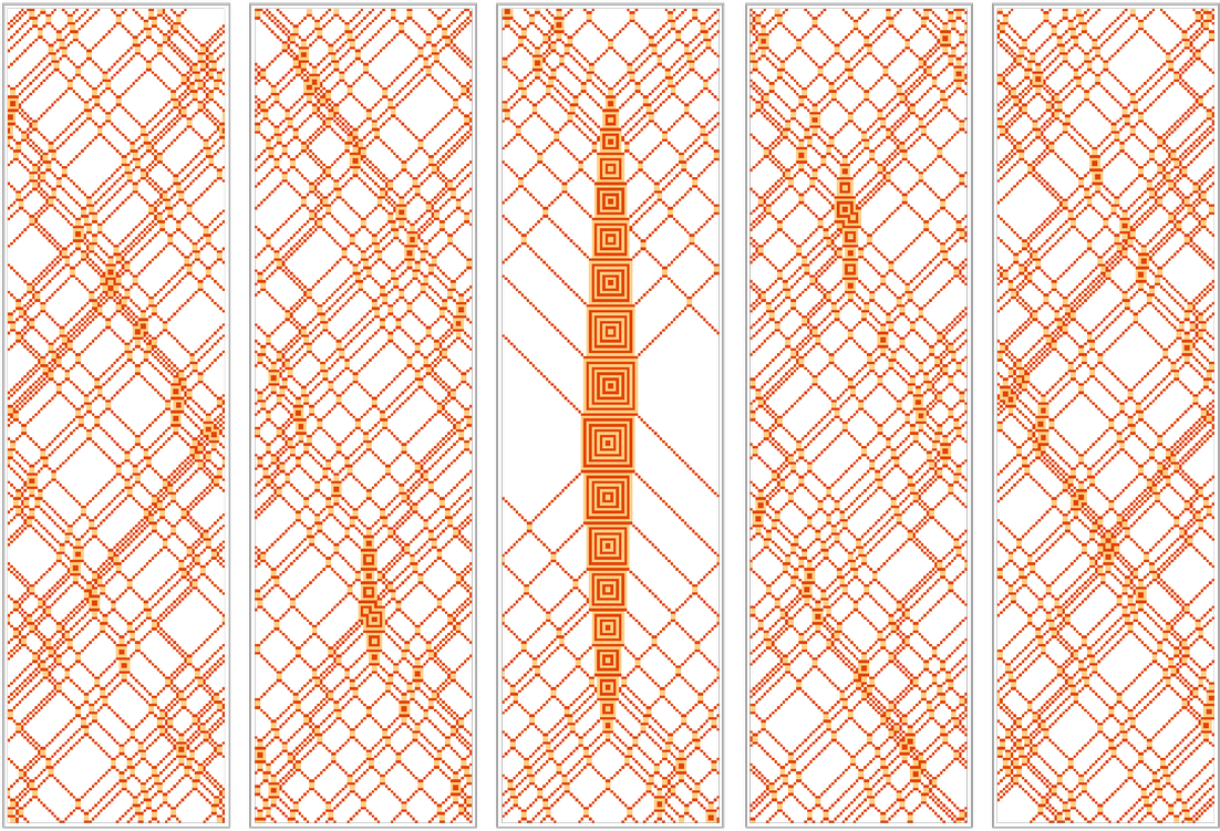
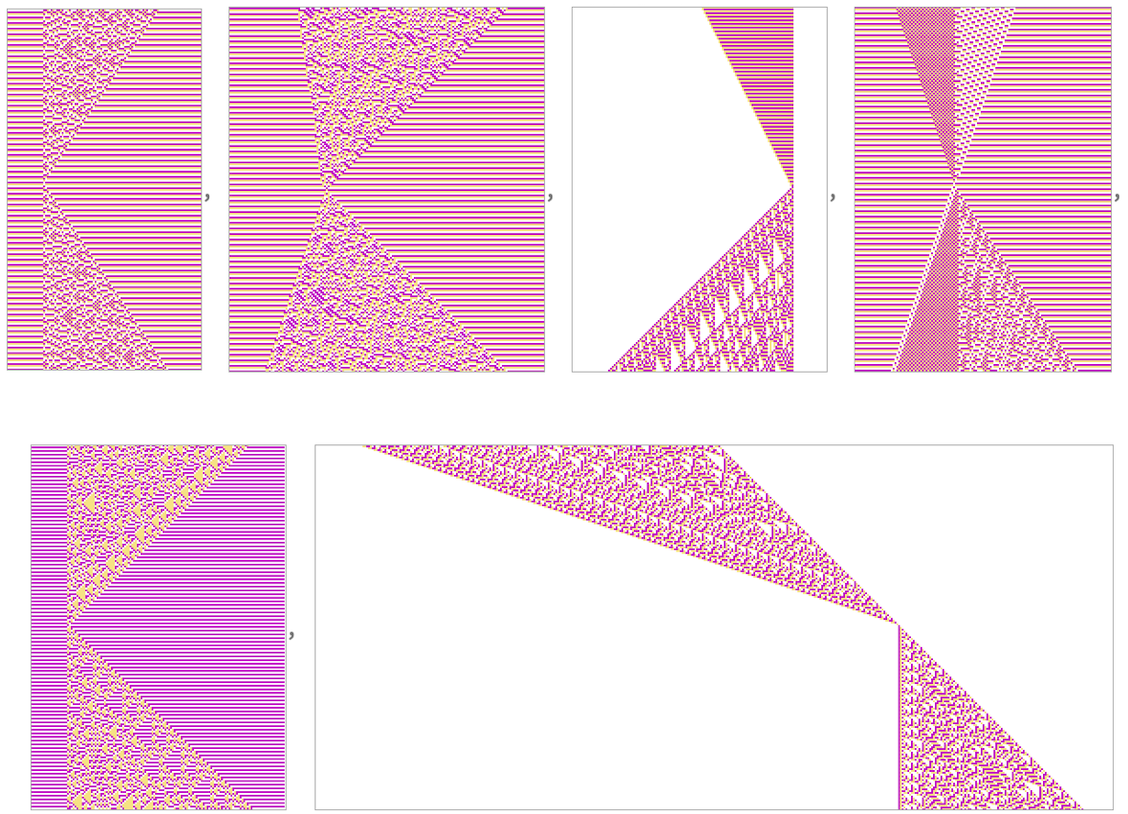
Let’s look again at rule 30. We start it off with different initial states, but in each case it quickly evolves to look basically the same:
Yes, the details of the patterns that emerge depend on the initial conditions. But the point is that the overall form of what’s produced is always the same: the system has reached a kind of “computational equilibrium” whose overall features are independent of where it came from. Later, we’ll see that the rapid emergence of “computational equilibrium” is characteristic of what I long ago identified as “class 3 systems”—and it’s quite ubiquitous to systems with a wide range of underlying rules, microscopically reversible or not.
That’s not to say that microscopic reversibility is irrelevant to “Second-Law-like” behavior. In what I called class 1 and class 2 systems the force of irreversibility in the underlying rules is strong enough that it overcomes computational irreducibility, and the systems ultimately evolve not to a “computational equilibrium” that looks random but rather to a definite, predictable end state:

How common is microscopic reversibility? In some types of rules it’s basically always there, by construction. But in other cases microscopically reversible rules represent just a subset of possible rules of a given type. For example, for block cellular automata with k colors and blocks of size b, there are altogether (kb)kb possible rules, of which kb! are reversible (i.e. of all mappings between possible blocks, only those that are permutations correspond to reversible rules). Among reversible rules, some—like the particle cellular automaton rule above—are “self-inverses”, in the sense that the forward and backward versions of the rule are the same.
But a rule like this is still reversible
and there’s still a straightforward backward rule, but it’s not exactly the same as the forward rule:
Using the backward rule, we can again construct an initial state whose forward evolution seems “anti-thermodynamic”, but the detailed behavior of the whole system isn’t perfectly symmetric between forward and backward in time:

Basic mechanics—like for our hard-sphere gas—is reversible and “self-inverse”. But it’s known that in particle physics there are small deviations from time reversal invariance, so that the rules are not precisely self-inverse—though they are still reversible in the sense that there’s always both a unique successor and a unique predecessor to every state (and indeed in our Physics Project such reversibility is probably guaranteed to exist in the laws of physics assumed by any observer who “believes they are persistent in time”).
For block cellular automata it’s very easy to determine from the underlying rule whether the system is reversible (just look to see if the rule serves only to permute the blocks). But for something like an ordinary cellular automaton it’s more difficult to determine reversibility from the rule (and above one dimension the question of reversibility can actually be undecidable). Among the 256 2-color nearest-neighbor rules there are only 6 reversible examples, and they are all trivial. Among the 134,217,728 3-color nearest-neighbor rules, 1800 are reversible. Of the 82 of these rules that are self-inverse, all are trivial. But when the inverse rules are different, the behavior can be nontrivial:
Note that unlike with block cellular automata the inverse rule often involves a larger neighborhood than the forward rule. (So, for example, here 396 rules have r = 1 inverses, 612 have r = 2, 648 have r = 3 and 144 have r = 4.)
A notable variant on ordinary cellular automata are “second-order” ones, in which the value of a cell depends on its value two steps in the past:

With this approach, one can construct reversible second-order variants of all 256 “elementary cellular automata”:

Note that such second-order rules are equivalent to 4-color first-order nearest-neighbor rules:

Ergodicity and Global Behavior
Whenever there’s a system with deterministic rules and a finite total number of states, it’s inevitable that the evolution of the system will eventually repeat. Sometimes the repetition period—or “recurrence time”—will be fairly short

and sometimes it’s much longer:

In general we can make a state transition graph that shows how each possible state of the system transitions to another under the rules. For a reversible system this graph consists purely of cycles in which each state has a unique successor and a unique predecessor. For a size-4 version of the system we’re studying here, there are a total of 2 ✕ 34 = 162 possible states (the factor 2 comes from the even/odd “phases” of the block cellular automaton)—and the state transition graph for this system is:

For a non-reversible system—like rule 30—the state transition graph (here shown for sizes 4 and 8) also includes “transient trees” of states that can be visited only once, on the way to a cycle:

In the past one of the key ideas for the origin of Second-Law-like behavior was ergodicity. And in the discrete-state systems we’re discussing here the definition of perfect ergodicity is quite straightforward: ergodicity just implies that the state transition graph must consist not of many cycles, but instead purely of one big cycle—so that whatever state one starts from, one’s always guaranteed to eventually visit every possible other state.
But why is this relevant to the Second Law? Well, we’ve said that the Second Law is about “degradation” from “special states” to “typical states”. And if one’s going to “do the ergodic thing” of visiting all possible states, then inevitably most of the states we’ll at least eventually pass through will be “typical”.
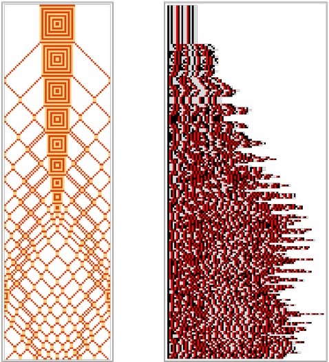
But on its own, this definitely isn’t enough to explain “Second-Law behavior” in practice. In an example like the following, one sees rapid “degradation” of a simple initial state to something “random” and “typical”:

But of the 2 ✕ 380 ≈ 1038 possible states that this system would eventually visit if it were ergodic, there are still a huge number that we wouldn’t consider “typical” or “random”. For example, just knowing that the system is eventually ergodic doesn’t tell one that it wouldn’t start off by painstakingly “counting down” like this, “keeping the action” in a tightly organized region:

So somehow there’s more than ergodicity that’s needed to explain the “degradation to randomness” associated with “typical Second-Law behavior”. And, yes, in the end it’s going to be a computational story, connected to computational irreducibility and its relationship to observers like us. But before we get there, let’s talk some more about “global structure”, as captured by things like state transition diagrams.
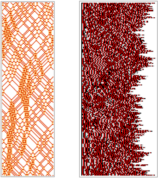
Consider again the size-4 case above. The rules are such that they conserve the number of “particles” (i.e. non-white cells). And this means that the states of the system necessarily break into separate “sectors” for different particle numbers. But even with a fixed number of particles, there are typically quite a few distinct cycles:

The system we’re using here is too small for us to be able to convincingly identify “simple” versus “typical” or “random” states, though for example we can see that only a few of the cycles have the simplifying feature of left-right symmetry.
Going to size 6 one begins to get a sense that there are some “always simple” cycles, as well as others that involve “more typical” states:

At size 10 the state transition graph for “4-particle” states has the form

and the longer cycles are:

It’s notable that most of the longest (“closest-to-ergodicity”) cycles look rather “simple and deliberate” all the way through. The “more typical and random” behavior seems to be reserved here for shorter cycles.
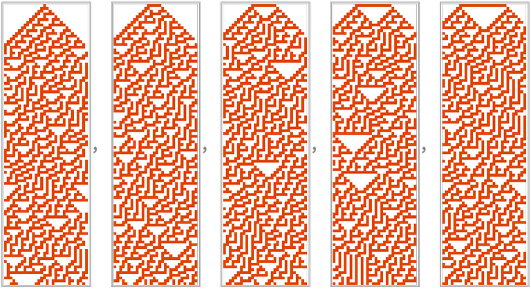
But in studying “Second Law behavior” what we’re mostly interested in is what happens from initially orderly states. Here’s an example of the results for progressively larger “blobs” in a system of size 30:

To get some sense of how the “degradation to randomness” proceeds, we can plot how the maximum blob size evolves in each case:

For some of the initial conditions one sees “thermodynamic-like” behavior, though quite often it’s overwhelmed by “freezing”, fluctuations, recurrences, etc. In all cases the evolution must eventually repeat, but the “recurrence times” vary widely (the longest—for a width-13 initial blob—being 861,930):

Let’s look at what happens in these recurrences, using as an example a width-17 initial blob—whose evolution begins:

As the picture suggests, the initial “large blob” quickly gets at least somewhat degraded, though there continue to be definite fluctuations visible:

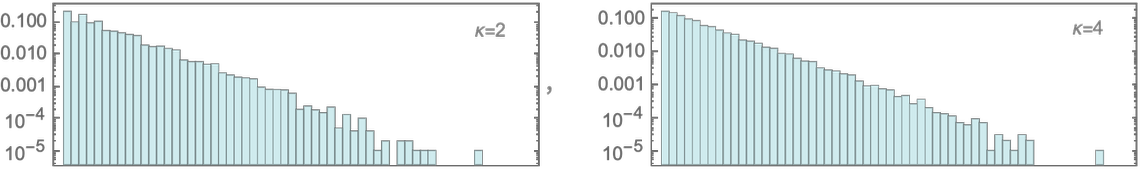
If one keeps going long enough, one reaches the recurrence time, which in this case is 155,150 steps. Looking at the maximum blob size through a “whole cycle” one sees many fluctuations:

Most are small—as illustrated here with ordinary and logarithmic histograms:

But some are large. And for example at half the full recurrence time there is a fluctuation

that involves an “emergent blob” as wide as in the initial condition—that altogether lasts around 280 steps:

There are also “runner-up” fluctuations with various forms—that reach “blob width 15” and occur more or less equally spaced throughout the cycle:

It’s notable that clear Second-Law-like behavior occurs even in a size-30 system. But if we go, say, to a size-80 system it becomes even more obvious

and one sees rapid and systematic evolution towards an “equilibrium state” with fairly small fluctuations:

It’s worth mentioning again that the idea of “reaching equilibrium” doesn’t depend on the particulars of the rule we’re using—and in fact it can happen more rapidly in other reversible block cellular automata where there are no “particle conservation laws” to slow things down:

In such rules there also tend to be fewer, longer cycles in the state transition graph, as this comparison for size 6 with the “delayed particle” rule suggests:

But it’s important to realize that the “approach to equilibrium” is its own—computational—phenomenon, not directly related to long cycles and concepts like ergodicity. And indeed, as we mentioned above, it also doesn’t depend on built-in reversibility in the rules, so one sees it even in something like rule 30:
How Random Does It Get?
At an everyday level, the core manifestation of the Second Law is the tendency of things to “degrade” to randomness. But just how random is the randomness? One might think that anything that is made by a simple-to-describe algorithm—like the pattern of rule 30 or the digits of π—shouldn’t really be considered “random”. But for the purpose of understanding our experience of the world what matters is not what is “happening underneath” but instead what our perception of it is. So the question becomes: when we see something produced, say by rule 30 or by π, can we recognize regularities in it or not?
And in practice what the Second Law asserts is that systems will tend to go from states where we can recognize regularities to ones where we cannot. And the point is that this phenomenon is something ubiquitous and fundamental, arising from core computational ideas, in particular computational irreducibility.
But what does it mean to “recognize regularities”? In essence it’s all about seeing if we can find succinct ways to summarize what we see—or at least the aspects of what we see that we care about. In other words, what we’re interested in is finding some kind of compressed representation of things. And what the Second Law is ultimately about is saying that even if compression works at first, it won’t tend to keep doing so.
As a very simple example, let’s consider doing compression by essentially “representing our data as a sequence of blobs”—or, more precisely, using run-length encoding to represent sequences of 0s and 1s in terms of lengths of successive runs of identical values. For example, given the data
we split into runs of identical values
then as a “compressed representation” just give the length of each run
which we can finally encode as a sequence of binary numbers with base-3 delimiters:
“Transforming” our “particle cellular automaton” in this way we get:
The “simple” initial conditions here are successfully compressed, but the later “random” states are not. Starting from a random initial condition, we don’t see any significant compression at all:
What about other methods of compression? A standard approach involves looking at blocks of successive values on a given step, and asking about the relative frequencies with which different possible blocks occur. But for the particular rule we are discussing here, there’s immediately an issue. The rule conserves the total number of non-white cells—so at least for size-1 blocks the frequency of such blocks will always be what it was for the initial conditions.
What about for larger blocks? This gives the evolution of relative frequencies of size-2 blocks starting from the simple initial condition above:
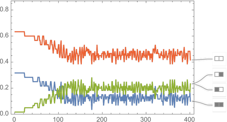
Arranging for exactly half the cells to be non-white, the frequencies of size-2 block converge towards equality:

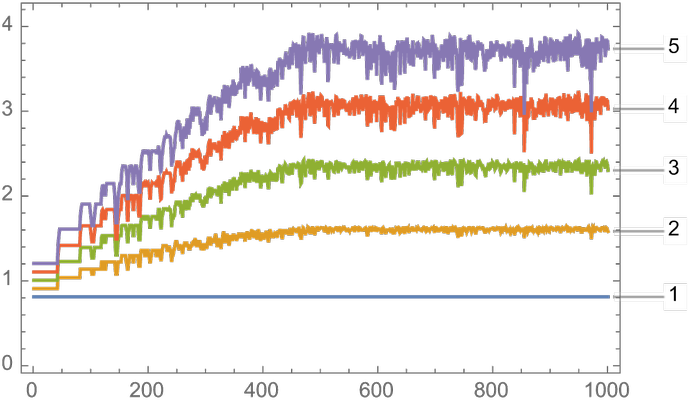
In general, the presence of unequal frequencies for different blocks allows the possibility of compression: much like in Morse code, one just has to use shorter codewords for more frequent blocks. How much compression is ultimately possible in this way can be found by computing –Σpi log pi for the probabilities pi of all blocks of a given length, which we see quickly converge to constant “equilibrium” values:
In the end we know that the initial conditions were “simple” and “special”. But the issue is whether whatever method we use for compression or for recognizing regularities is able to pick up on this. Or whether somehow the evolution of the system has sufficiently “encoded” the information about the initial condition that it’s no longer detectable. Clearly if our “method of compression” involved explicitly running the evolution of the system backwards, then it’d be possible to pick out the special features of the initial conditions. But explicitly running the evolution of the system requires doing lots of computational work.
So in a sense the question is whether there’s a shortcut. And, yes, one can try all sorts of methods from statistics, machine learning, cryptography and so on. But so far as one can tell, none of them make any significant progress: the “encoding” associated with the evolution of the system seems to just be too strong to “break”. Ultimately it’s hard to know for sure that there’s no scheme that can work. But any scheme must correspond to running some program. So a way to get a bit more evidence is just to enumerate “possible compression programs” and see what they do.
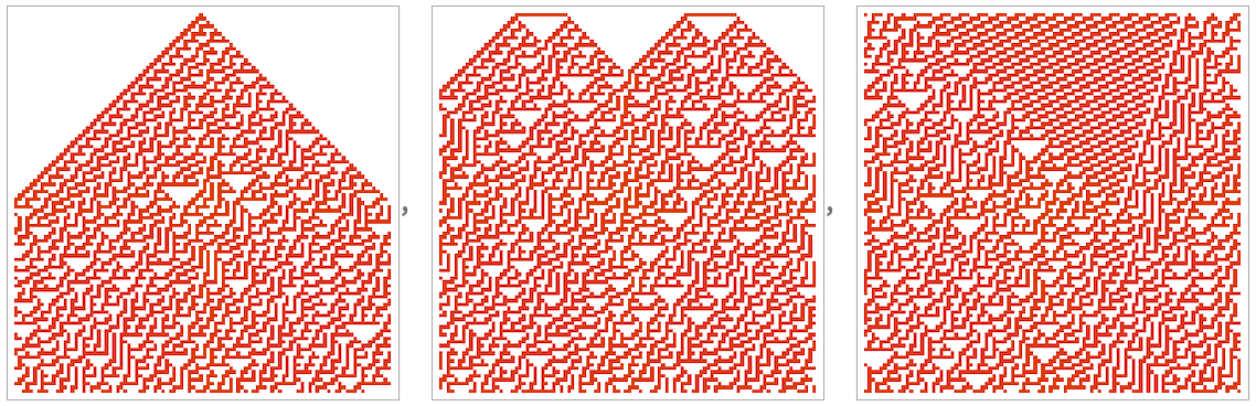
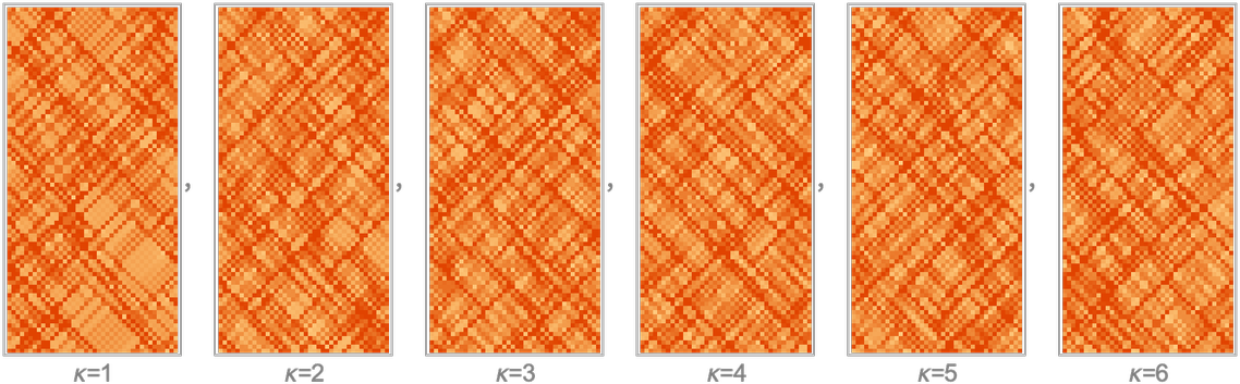
In particular, we can for example enumerate simple cellular automata, and see whether when run they produce “obviously different” results. Here’s what happens for a collection of different cellular automata when they are applied to a “simple initial condition”, to states obtained after 20 and 200 steps of evolution according to the particle cellular automaton rule and to an independently random state:
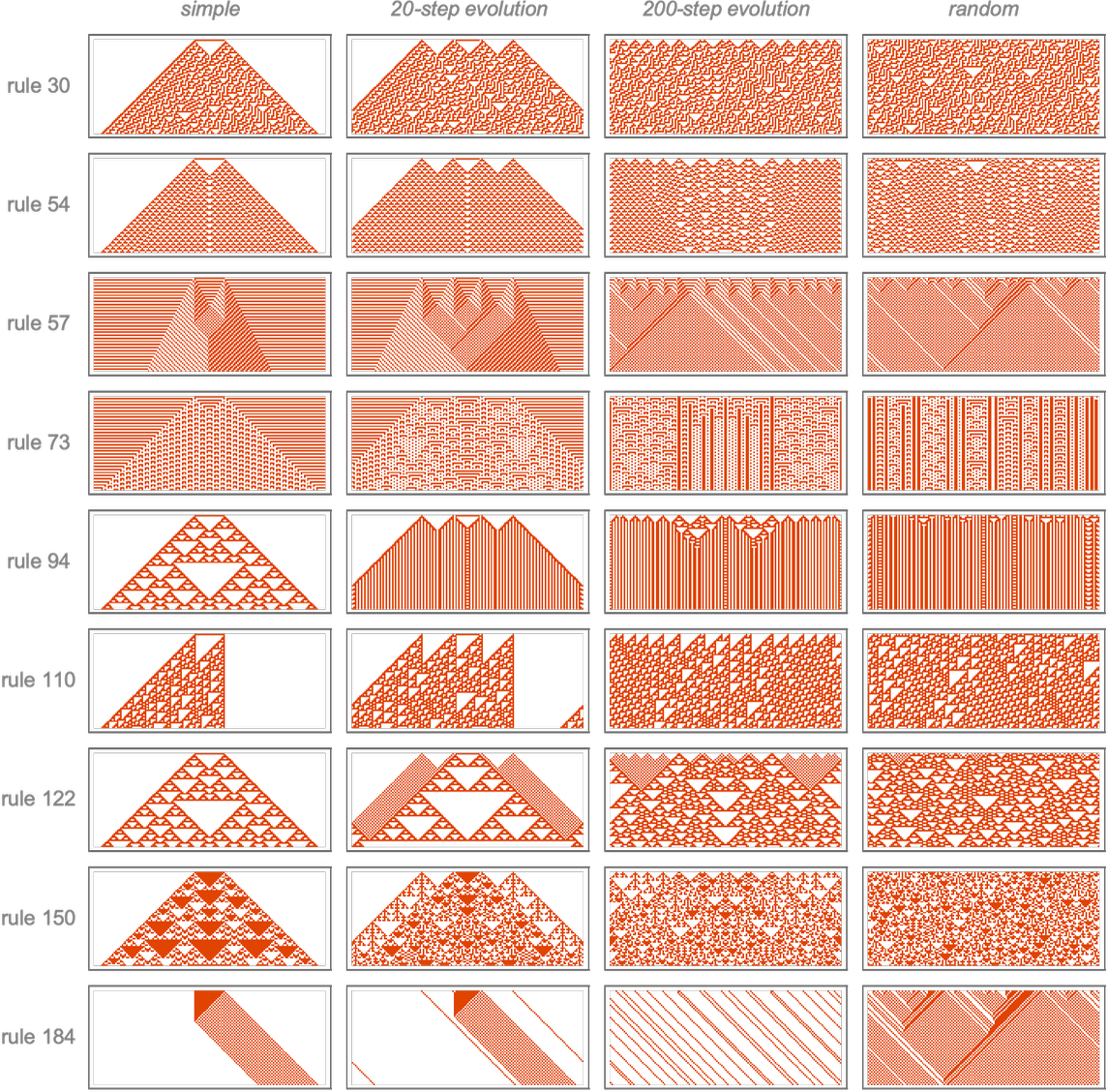
And, yes, in many cases the simple initial condition leads to “obviously different behavior”. But there’s nothing obviously different about the behavior obtained in the last two cases. Or, in other words, at least programs based on these simple cellular automata don’t seem to be able to “decode” the different origins of the third and fourth cases shown here.
What does all this mean? The fundamental point is that there seems to be enough computational irreducibility in the evolution of the system that no computationally bounded observer can “see through it”. And so—at least as far as a computationally bounded observer is concerned—“specialness” in the initial conditions is quickly “degraded” to an “equilibrium” state that “seems random”. Or, in other words, the computational process of evolution inevitably seems to lead to the core phenomenon of the Second Law.
The Concept of Entropy
“Entropy increases” is a common statement of the Second Law. But what does this mean, especially in our computational context? The answer is somewhat subtle, and understanding it will put us right back into questions of the interplay between computational irreducibility and the computational boundedness of observers.
When it was first introduced in the 1860s, entropy was thought of very much like energy, and was computed from ratios of heat content to temperature. But soon—particularly through work on gases by Boltzmann—there arose a quite different way of computing (and thinking about) entropy: in terms of the log of the number of possible states of a system. Later we’ll discuss the correspondence between these different ideas of entropy. But for now let’s consider what I view as the more fundamental definition based on counting states.
In the early days of entropy, when one imagined that—like in the cases of the hard-sphere gas—the parameters of the system were continuous, it could be mathematically complex to tease out any kind of discrete “counting of states”. But from what we’ve discussed here, it’s clear that the core phenomenon of the Second Law doesn’t depend on the presence of continuous parameters, and in something like a cellular automaton it’s basically straightforward to count discrete states.
But now we have to get more careful about our definition of entropy. Given any particular initial state, a deterministic system will always evolve through a series of individual states—so that there’s always only one possible state for the system, which means the entropy will always be exactly zero. (This is a lot muddier and more complicated when continuous parameters are considered, but in the end the conclusion is the same.)
So how do we get a more useful definition of entropy? The key idea is to think not about individual states of a system but instead about collections of states that we somehow consider “equivalent”. In a typical case we might imagine that we can’t measure all the detailed positions of molecules in a gas, so we look just at “coarse-grained” states in which we consider, say, only the number of molecules in particular overall bins or blocks.
The entropy can be thought of as counting the number of possible microscopic states of the system that are consistent with some overall constraint—like a certain number of particles in each bin. If the constraint talks specifically about the position of every particle, there’ll only be one microscopic state consistent with the constraints, and the entropy will be zero. But if the constraint is looser, there’ll often be many possible microscopic states consistent with it, and the entropy we define will be nonzero.
Let’s look at this in the context of our particle cellular automaton. Here’s a particular evolution, starting from a specific microscopic state, together with a sequence of “coarse grainings” of this evolution in which we keep track only of “overall particle density” in progressively larger blocks:

The very first “coarse graining” here is particularly trivial: all it’s doing is to say whether a “particle is present” or not in each cell—or, in other words, it’s showing every particle but ignoring whether it’s “light” or “dark”. But in making this and the other coarse-grained pictures we’re always starting from the single “underlying microscopic evolution” that’s shown and just “adding coarse graining after the fact”.
But what if we assume that all we ever know about the system is a coarse-grained version? Say we look at the “particle-or-not” case. At a coarse-grained level the initial condition just says there are 6 particles present. But it doesn’t say if each particle is light or dark, and actually there are 26 = 64 possible microscopic configurations. And the point is that each of these microscopic configurations has its own evolution:

But now we can consider coarse graining things. All 64 initial conditions are—by construction—equivalent under particle-or-not coarse graining:

But after just one step of evolution, different initial “microstates” can lead to different coarse-grained evolutions:

In other words, a single coarse-grained initial condition “spreads out” after just one step to several coarse-grained states:
After another step, a larger number of coarse-grained states are possible:
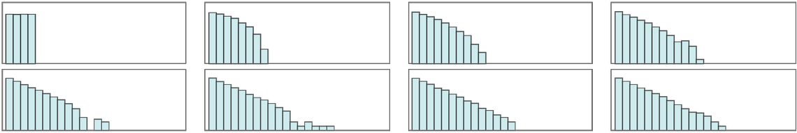
And in general the number of distinct coarse-grained states that can be reached grows fairly rapidly at first, though soon saturates, showing just fluctuations thereafter:

But the coarse-grained entropy is basically just proportional to the log of this quantity, so it too will show rapid growth at first, eventually leveling off at an “equilibrium” value.
The framework of our Physics Project makes it natural to think of coarse-grained evolution as a multicomputational process—in which a given coarse-grained state has not just a single successor, but in general multiple possible successors. For the case we’re considering here, the multiway graph representing all possible evolution paths is then:
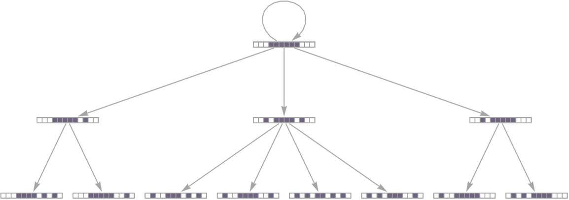
The branching here reflects a spreading out in coarse-grained state space, and an increase in coarse-grained entropy. If we continue longer—so that the system begins to “approach equilibrium”—we’ll start to see some merging as well

as a less “time-oriented” graph layout makes clear:

But the important point is that in its “approach to equilibrium” the system in effect rapidly “spreads out” in coarse-grained state space. Or, in other words, the number of possible states of the system consistent with a particular coarse-grained initial condition increases, corresponding to an increase in what one can consider to be the entropy of the system.
There are many possible ways to set up what we might view as “coarse graining”. An example of another possibility is to focus on the values of a particular block of cells, and then to ignore the values of all other cells. But it typically doesn’t take long for the effects of other cells to “seep into” the block we’re looking at:

So what is the bigger picture? The basic point is that insofar as the evolution of each individual microscopic state “leads to randomness”, it’ll tend to end up in a different “coarse-grained bin”. And the result is that even if one starts with a tightly defined coarse-grained description, it’ll inevitably tend to “spread out”, thereby encompassing more states and increasing the entropy.
In a sense, looking at entropy and coarse graining is just a less direct way to detect that a system tends to “produce effective randomness”. And while it may have seemed like a convenient formalism when one was, for example, trying to tease things out from systems with continuous variables, it now feels like a rather indirect way to get at the core phenomenon of the Second Law.
It’s useful to understand a few more connections, however. Let’s say one’s trying to work out the average value of something (say particle density) in a system. What do we mean by “average”? One possibility is that we take an “ensemble” of possible states of the system, then find the average across these. But another possibility is that we instead look at the average across successive states in the evolution of the system. The “ergodic hypothesis” is that the ensemble average will be the same as the time average.
One way this would—at least eventually—be guaranteed is if the evolution of the system is ergodic, in the sense that it eventually visits all possible states. But as we saw above, this isn’t something that’s particularly plausible for most systems. But it also isn’t necessary. Because so long as the evolution of the system is “effectively random” enough, it’ll quickly “sample typical states”, and give essentially the same averages as one would get from sampling all possible states, but without having to laboriously visit all these states.
How does one tie all this down with rigorous, mathematical-style proofs? Well, it’s difficult. And in a first approximation not much progress has been made on this for more than a century. But having seen that the core phenomenon of the Second Law can be reduced to an essentially purely computational statement, we’re now in a position to examine this in a different—and I think ultimately very clarifying—way.
Why the Second Law Works
At its core the Second Law is essentially the statement that “things tend to get more random”. And in a sense the ultimate driver of this is the surprising phenomenon of computational irreducibility I identified in the 1980s—and the remarkable fact that even from simple initial conditions simple computational rules can generate behavior of great complexity. But there are definitely additional nuances to the story.
For example, we’ve seen that—particularly in a reversible system—it’s always in principle possible to set up initial conditions that will evolve to “magically produce” whatever “simple” configuration we want. And when we say that we generate “apparently random” states, our “analyzer of randomness” can’t go in and invert the computational process that generated the states. Similarly, when we talk about coarse-grained entropy and its increase, we’re assuming that we’re not inventing some elaborate coarse-graining procedure that’s specially set up to pick out collections of states with “special” behavior.
But there’s really just one principle that governs all these things: that whatever method we have to prepare or analyze states of a system is somehow computationally bounded. This isn’t as such a statement of physics. Rather, it’s a general statement about observers, or, more specifically, observers like us.
We could imagine some very detailed model for an observer, or for the experimental apparatus they use. But the key point is that the details don’t matter. Really all that matters is that the observer is computationally bounded. And it’s then the basic computational mismatch between the observer and the computational irreducibility of the underlying system that leads us to “experience” the Second Law.
At a theoretical level we can imagine an “alien observer”—or even an observer with technology from our own future—that would not have the same computational limitations. But the point is that insofar as we are interested in explaining our own current experience, and our own current scientific observations, what matters is the way we as observers are now, with all our computational boundedness. And it’s then the interplay between this computational boundedness, and the phenomenon of computational irreducibility, that leads to our basic experience of the Second Law.
At some level the Second Law is a story of the emergence of complexity. But it’s also a story of the emergence of simplicity. For the very statement that things go to a “completely random equilibrium” implies great simplification. Yes, if an observer could look at all the details they would see great complexity. But the point is that a computationally bounded observer necessarily can’t look at those details, and instead the features they identify have a certain simplicity.
And so it is, for example, that even though in a gas there are complicated underlying molecular motions, it’s still true that at an overall level a computationally bounded observer can meaningfully discuss the gas—and make predictions about its behavior—purely in terms of things like pressure and temperature that don’t probe the underlying details of molecular motions.
In the past one might have thought that anything like the Second Law must somehow be specific to systems made from things like interacting particles. But in fact the core phenomenon of the Second Law is much more general, and in a sense purely computational, depending only on the basic computational phenomenon of computational irreducibility, together with the fundamental computational boundedness of observers like us.
And given this generality it’s perhaps not surprising that the core phenomenon appears far beyond where anything like the Second Law has normally been considered. In particular, in our Physics Project it now emerges as fundamental to the structure of space itself—as well as to the phenomenon of quantum mechanics. For in our Physics Project we imagine that at the lowest level everything in our universe can be represented by some essentially computational structure, conveniently described as a hypergraph whose nodes are abstract “atoms of space”. This structure evolves by following rules, whose operation will typically show all sorts of computational irreducibility. But now the question is how observers like us will perceive all this. And the point is that through our limitations we inevitably come to various “aggregate” conclusions about what’s going on. It’s very much like with the gas laws and their broad applicability to systems involving different kinds of molecules. Except that now the emergent laws are about spacetime and correspond to the equations of general relativity.
But the basic intellectual structure is the same. Except that in the case of spacetime, there’s an additional complication. In thermodynamics, we can imagine that there’s a system we’re studying, and the observer is outside it, “looking in”. But when we’re thinking about spacetime, the observer is necessarily embedded within it. And it turns out that there’s then one additional feature of observers like us that’s important. Beyond the statement that we’re computationally bounded, it’s also important that we assume that we’re persistent in time. Yes, we’re made of different atoms of space at different moments. But somehow we assume that we have a coherent thread of experience. And this is crucial in deriving our familiar laws of physics.
We’ll talk more about it later, but in our Physics Project the same underlying setup is also what leads to the laws of quantum mechanics. Of course, quantum mechanics is notable for the apparent randomness associated with observations made in it. And what we’ll see later is that in the end the same core phenomenon responsible for randomness in the Second Law also appears to be what’s responsible for randomness in quantum mechanics.
The interplay between computational irreducibility and computational limitations of observers turns out to be a central phenomenon throughout the multicomputational paradigm and its many emerging applications. It’s core to the fact that observers can experience computationally reducible laws in all sorts of samplings of the ruliad. And in a sense all of this strengthens the story of the origins of the Second Law. Because it shows that what might have seemed like arbitrary features of observers are actually deep and general, transcending a vast range of areas and applications.
But even given the robustness of features of observers, we can still ask about the origins of the whole computational phenomenon that leads to the Second Law. Ultimately it begins with the Principle of Computational Equivalence, which asserts that systems whose behavior is not obviously simple will tend to be equivalent in their computational sophistication. The Principle of Computational Equivalence has many implications. One of them is computational irreducibility, associated with the fact that “analyzers” or “predictors” of a system cannot be expected to have any greater computational sophistication than the system itself, and so are reduced to just tracing each step in the evolution of a system to find out what it does.
Another implication of the Principle of Computational Equivalence is the ubiquity of computation universality. And this is something we can expect to see “underneath” the Second Law. Because we can expect that systems like the particle cellular automaton—or, for that matter, the hard-sphere gas—will be provably capable of universal computation. Already it’s easy to see that simple logic gates can be constructed from configurations of particles, but a full demonstration of computation universality will be considerably more elaborate. And while it’d be nice to have such a demonstration, there’s still more that’s needed to establish full computational irreducibility of the kind the Principle of Computational Equivalence implies.
As we’ve seen, there are a variety of “indicators” of the operation of the Second Law. Some are based on looking for randomness or compression in individual states. Others are based on computing coarse grainings and entropy measures. But with the computational interpretation of the Second Law we can expect to translate such indicators into questions in areas like computational complexity theory.
At some level we can think of the Second Law as being a consequence of the dynamics of a system so “encrypting” the initial conditions of a system that no computations available to an “observer” can feasibly “decrypt” it. And indeed as soon as one looks at “inverting” coarse-grained results one is immediately faced with fairly classic NP problems from computational complexity theory. (Establishing NP completeness in a particular case remains challenging, just like establishing computation universality.)
Textbook Thermodynamics
In our discussion here, we’ve treated the Second Law of thermodynamics primarily as an abstract computational phenomenon. But when thermodynamics was historically first being developed, the computational paradigm was still far in the future, and the only way to identify something like the Second Law was through its manifestations in terms of physical concepts like heat and temperature.
The First Law of thermodynamics asserted that heat was a form of energy, and that overall energy was conserved. The Second Law then tried to characterize the nature of the energy associated with heat. And a core idea was that this energy was somehow incoherently spread among a large number of separate microscopic components. But ultimately thermodynamics was always a story of energy.
But is energy really a core feature of thermodynamics or is it merely “scaffolding” relevant for its historical development and early practical applications? In the hard-sphere gas example that we started from above, there’s a pretty clear notion of energy. But quite soon we largely abstracted energy away. Though in our particle cellular automaton we do still have something somewhat analogous to energy conservation: we have conservation of the number of non-white cells.
In a traditional physical system like a gas, temperature gives the average energy per degree of freedom. But in something like our particle cellular automaton, we’re effectively assuming that all particles always have the same energy—so there is for example no way to “change the temperature”. Or, put another way, what we might consider as the energy of the system is basically just given by the number of particles in the system.
Does this simplification affect the core phenomenon of the Second Law? No. That’s something much stronger, and quite independent of these details. But in the effort to make contact with recognizable “textbook thermodynamics”, it’s useful to consider how we’d add in ideas like heat and temperature.
In our discussion of the Second Law, we’ve identified entropy with the log of the number states consistent with a constraint. But more traditional thermodynamics involves formulas like
When the Second Law was first introduced, there were several formulations given, all initially referencing energy. One formulation stated that “heat does not spontaneously go from a colder body to a hotter”. And even in our particle cellular automaton we can see a fairly direct version of this. Our proxy for “temperature” is density of particles. And what we observe is that an initial region of higher density tends to “diffuse” out:
Another formulation of the Second Law talks about the impossibility of systematically “turning heat into mechanical work”. At a computational level, the analog of “mechanical work” is systematic, predictable behavior. So what this is saying is again that systems tend to generate randomness, and to “remove predictability”.
In a sense this is a direct reflection of computational irreducibility. To get something that one can “harness as mechanical work” one needs something that one can readily predict. But the whole point is that the presence of computational irreducibility makes prediction take an irreducible amount of computational work—that is beyond the capabilities of an “observer like us”.
Closely related is the statement that it’s not possible to make a perpetual motion machine (“of the second kind”, i.e. violating the Second Law), that continually “makes systematic motion” from “heat”. In our computational setting this would be like extracting a systematic, predictable sequence of bits from our particle cellular automaton, or from something like rule 30. And, yes, if we had a device that could for example systematically predict rule 30, then it would be straightforward, say, “just to pick out black cells”, and effectively to derive a predictable sequence. But computational irreducibility implies that we won’t be able to do this, without effectively just directly reproducing what rule 30 does, which an “observer like us” doesn’t have the computational capability to do.
Much of the textbook discussion of thermodynamics is centered around the assumption of “equilibrium”—or something infinitesimally close to it—in which one assumes that a system behaves “uniformly and randomly”. Indeed, the Zeroth Law of thermodynamics is essentially the statement that “statistically unique” equilibrium can be achieved, which in terms of energy becomes a statement that there is a unique notion of temperature.
Once one has the idea of “equilibrium”, one can then start to think of its properties as purely being functions of certain parameters—and this opens up all sorts of calculus-based mathematical opportunities. That anything like this makes sense depends, however, yet again on “perfect randomness as far as the observer is concerned”. Because if the observer could notice a difference between different configurations, it wouldn’t be possible to treat all of them as just being “in the equilibrium state”.
Needless to say, while the intuition of all this is made rather clear by our computational view, there are details to be filled in when it comes to any particular mathematical formulation of features of thermodynamics. As one example, let’s consider a core result of traditional thermodynamics: the Maxwell–Boltzmann exponential distribution of energies for individual particles or other degrees of freedom.
To set up a discussion of this, we need to have a system where there can be many possible microscopic amounts of energy, say, associated with some kind of idealized particles. Then we imagine that in “collisions” between such particles energy is exchanged, but the total is always conserved. And the question is how energy will eventually be distributed among the particles.
As a first example, let’s imagine that we have a collection of particles which evolve in a series of steps, and that at each step particles are paired up at random to “collide”. And, further, let’s assume that the effect of the collision is to randomly redistribute energy between the particles, say with a uniform distribution.
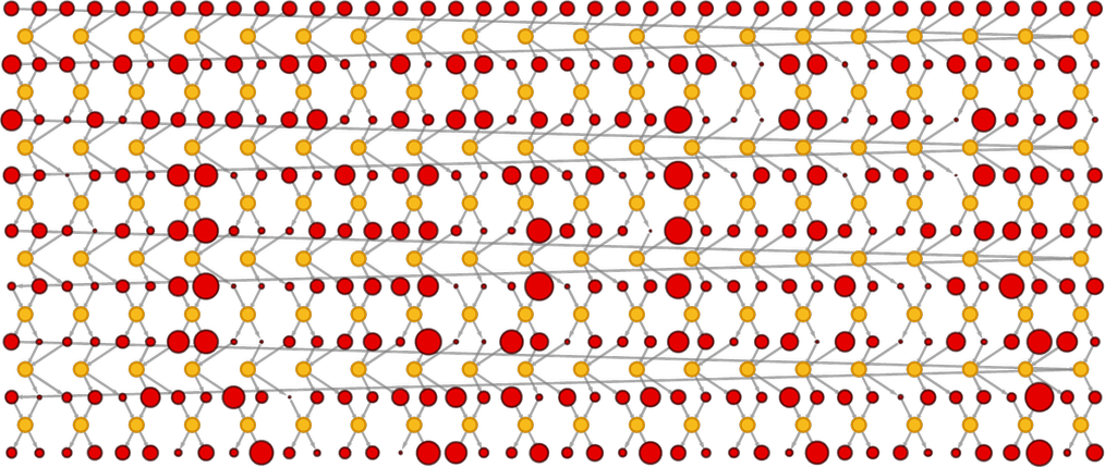
We can represent this process using a token-event graph, where the events (indicated here in yellow) are the collisions, and the tokens (indicated here in red) represent states of particles at each step. The energy of the particles is indicated here by the size of the “token dots”:
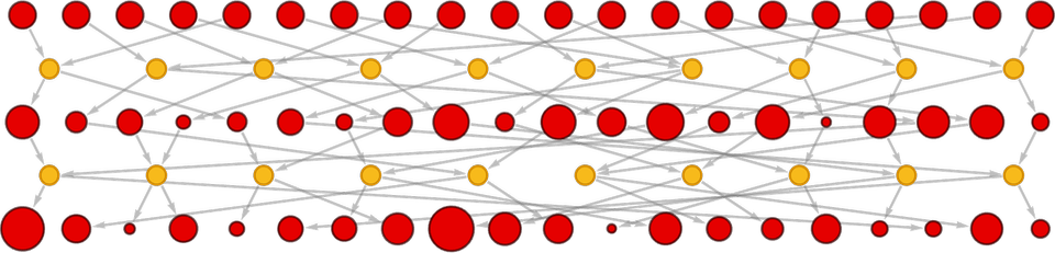
Continuing this a few more steps we get:
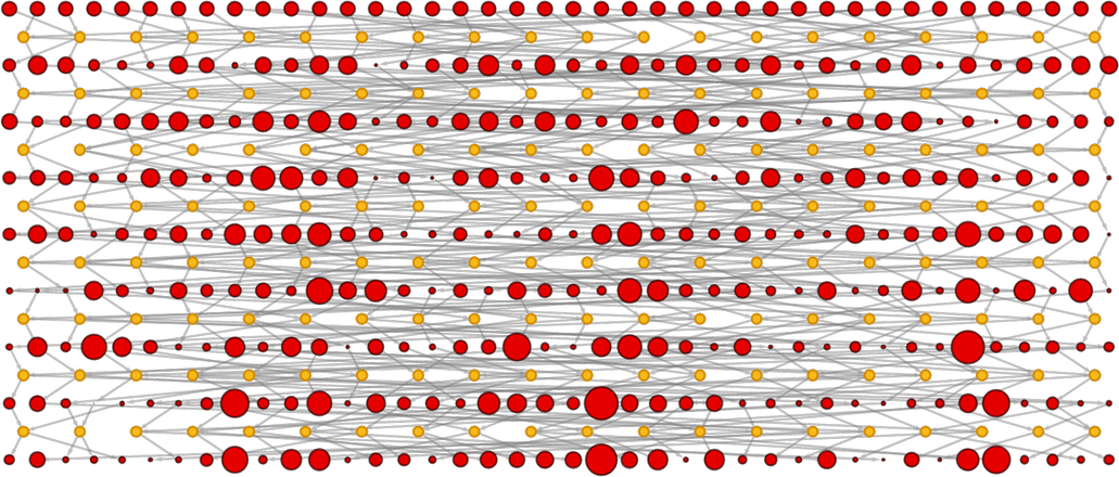
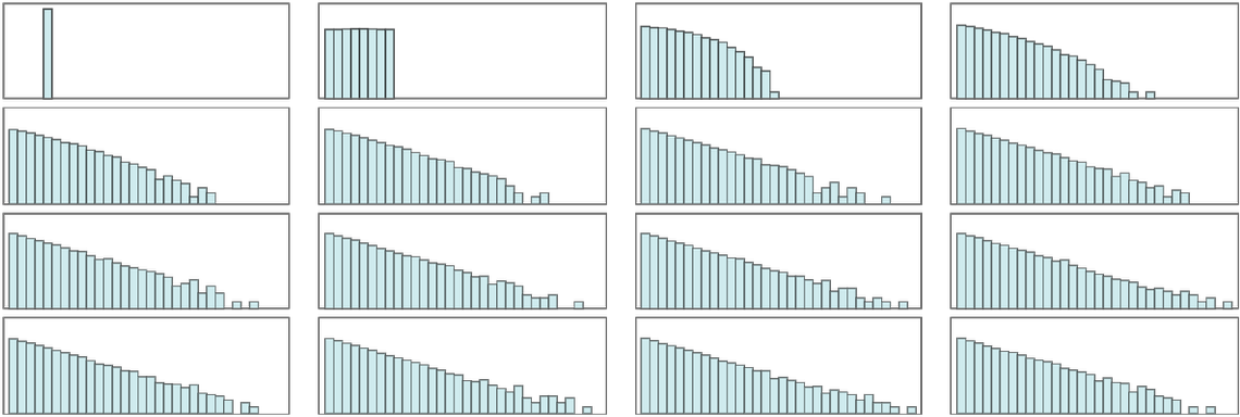
At the beginning we started with all particles having equal energies. But after a number of steps the particles have a distribution of energies—and the distribution turns out to be accurately exponential, just like the standard Maxwell–Boltzmann distribution:
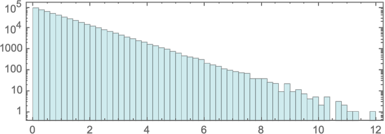
If we look at the distribution on successive steps we see rapid evolution to the exponential form:
Why we end up with an exponential is not hard to see. In the limit of enough particles and enough collisions, one can imagine approximating everything purely in terms of probabilities (as one does in deriving Boltzmann transport equations, basic SIR models in epidemiology, etc.) Then if the probability for a particle to have energy E is ƒ(E), in every collision once the system has “reached equilibrium” one must have ƒ(E1)ƒ(E2) = ƒ(E3)ƒ(E4) where E1 + E2 = E3 + E4—and the only solution to this is ƒ(E) ∼ e–β E.
In the example we’ve just given, there’s in effect “immediate mixing” between all particles. But what if we set things up more like in a cellular automaton—with particles only colliding with their local neighbors in space? As an example, let’s say we have our particles arranged on a line, with alternating pairs colliding at each step in analogy to a block cellular automaton (the long-range connections represent wraparound of our lattice):
In the picture above we’ve assumed that in each collision energy is randomly redistributed between the particles. And with this assumption it turns out that we again rapidly evolve to an exponential energy distribution:

But now that we have a spatial structure, we can display what’s going on in more of a cellular automaton style—where here we’re showing results for 3 different sequences of random energy exchanges:

And once again, if we run long enough, we eventually get an exponential energy distribution for the particles. But note that the setup here is very different from something like rule 30—because we’re continuously injecting randomness from the outside into the system. And as a minimal way to avoid this, consider a model where at each collision the particles get fixed fractions

Here’s what happens with energy concentrated into a few particles

and with random initial energies:

And in all cases the system eventually evolves to a “pure checkerboard” in which the only particle energies are (1 – α)/2 and (1 + α)/2. (For α = 0 the system corresponds to a discrete version of the diffusion equation.) But if we look at the structure of the system, we can think of it as a continuous block cellular automaton. And as with other cellular automata, there are lots of possible rules that don’t lead to such simple behavior.
In fact, all we need do is allow α to depend on the energies E1 and E2 of colliding pairs of particles (or, here, the values of cells in each block). As an example, let’s take

And with this setup we once again often see “rule-30-like behavior” in which effectively quite random behavior is generated even without any explicit injection of randomness from outside (the lower panels start at step 1000):
The underlying construction of the rule ensures that total energy is conserved. But what we see is that the evolution of the system distributes it across many elements. And at least if we use random initial conditions
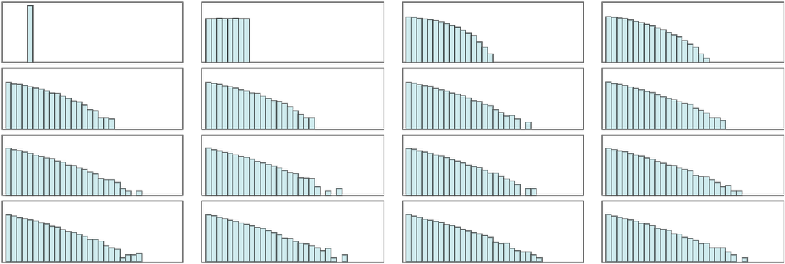
we eventually in all cases see an exponential distribution of energy values (with simple initial conditions it can be more complicated):
The evolution towards this is very much the same as in the systems above. In a sense it depends only on having a suitably randomized energy-conserving collision process, and it takes only a few steps to go from a uniform initial distribution energy to an accurately exponential one:
So how does this all work in a “physically realistic” hard-sphere gas? Once again we can create a token-event graph, where the events are collisions, and the tokens correspond to periods of free motion of particles. For a simple 1D “Newton’s cradle” configuration, there is an obvious correspondence between the evolution in “spacetime”, and the token-event graph:

But we can do exactly the same thing for a 2D configuration. Indicating the energies of particles by the sizes of tokens we get (excluding wall collisions, which don’t affect particle energy)

where the “filmstrip” at the side gives snapshots of the evolution of the system. (Note that in this system, unlike the ones above, there aren’t definite “steps” of evolution; the collisions just happen “asynchronously” at times determined by the dynamics.)
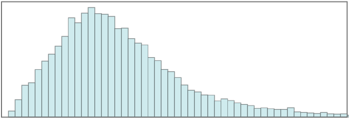
In the initial condition we’re using here, all particles have the same energy. But when we run the system we find that the energy distribution for the particles rapidly evolves to the standard exponential form (though note that here successive panels are “snapshots”, not “steps”):

And because we’re dealing with “actual particles”, we can look not only at their energies, but also at their speeds (related simply by E = 1/2 m v2). When we look at the distribution of speeds generated by the evolution, we find that it has the classic Maxwellian form:
And it’s this kind of final or “equilibrium” result that’s what’s mainly discussed in typical textbooks of thermodynamics. Such books also tend to talk about things like tradeoffs between energy and entropy, and define things like the (Helmholtz) free energy F = U – T S (where U is internal energy, T is temperature and S is entropy) that are used in answering questions like whether particular chemical reactions will occur under certain conditions.
But given our discussion of energy here, and our earlier discussion of entropy, it’s at first quite unclear how these quantities might relate, and how they can trade off against each other, say in the formula for free energy. But in some sense what connects energy to the standard definition of entropy in terms of the logarithm of the number of states is the Maxwell–Boltzmann distribution, with its exponential form. In the usual physical setup, the Maxwell–Boltzmann distribution is basically e(–E/kT), where T is the temperature, and kT is the average energy.
But now imagine we’re trying to figure out whether some process—say a chemical reaction—will happen. If there’s an energy barrier, say associated with an energy difference Δ, then according to the Maxwell–Boltzmann distribution there’ll be a probability proportional to e(–Δ/kT) for molecules to have a high enough energy to surmount that barrier. But the next question is how many configurations of molecules there are in which molecules will “try to surmount the barrier”. And that’s where the entropy comes in. Because if the number of possible configurations is Ω, the entropy S is given by k log Ω, so that in terms of S, Ω = e(S/k). But now the “average number of molecules which will surmount the barrier” is roughly given by
This argument is quite rough, but it captures the essence of what’s going on. And at first it might seem like a remarkable coincidence that there’s a logarithm in the definition of entropy that just “conveniently fits together” like this with the exponential in the Maxwell–Boltzmann distribution. But it’s actually not a coincidence at all. The point is that what’s really fundamental is the concept of counting the number of possible states of a system. But typically this number is extremely large. And we need some way to “tame” it. We could in principle use some slow-growing function other than log to do this. But if we use log (as in the standard definition of entropy) we precisely get the tradeoff with energy in the Maxwell–Boltzmann distribution.
There is also another convenient feature of using log. If two systems are independent, one with Ω1 states, and the other with Ω2 states, then a system that combines these (without interaction) will have Ω1, Ω2 states. And if S = k log Ω, then this means that the entropy of the combined state will just be the sum S1 + S2 of the entropies of the individual states. But is this fact actually “fundamentally independent” of the exponential character of the Maxwell–Boltzmann distribution? Well, no. Or at least it comes from the same mathematical idea. Because it’s the fact that in equilibrium the probability ƒ(E) is supposed to satisfy ƒ(E1)ƒ(E2) = ƒ(E3)ƒ(E4) when E1 + E2 = E3 + E4 that makes ƒ(E) have its exponential form. In other words, both stories are about exponentials being able to connect additive combination of one quantity with multiplicative combination of another.
Having said all this, though, it’s important to understand that you don’t need energy to talk about entropy. The concept of entropy, as we’ve discussed, is ultimately a computational concept, quite independent of physical notions like energy. In many textbook treatments of thermodynamics, energy and entropy are in some sense put on a similar footing. The First Law is about energy. The Second Law is about entropy. But what we’ve seen here is that energy is really a concept at a different level from entropy: it’s something one gets to “layer on” in discussing physical systems, but it’s not a necessary part of the “computational essence” of how things work.
(As an extra wrinkle, in the case of our Physics Project—as to some extent in traditional general relativity and quantum mechanics—there are some fundamental connections between energy and entropy. In particular—related to what we’ll discuss below—the number of possible discrete configurations of spacetime is inevitably related to the “density” of events, which defines energy.)
Towards a Formal Proof of the Second Law
It would be nice to be able to say, for example, that “using computation theory, we can prove the Second Law”. But it isn’t as simple as that. Not least because, as we’ve seen, the validity of the Second Law depends on things like what “observers like us” are capable of. But we can, for example, formulate what the outline of a proof of the Second Law could be like, though to give a full formal proof we’d have to introduce a variety of “axioms” (essentially about observers) that don’t have immediate foundations in existing areas of mathematics, physics or computation theory.
The basic idea is that one imagines a state S of a system (which could just be a sequence of values for cells in something like a cellular automaton). One considers an “observer function” Θ which, when applied to the state S, gives a “summary” of S. (A very simple example would be the run-length encoding that we used above.) Now we imagine some “evolution function” Ξ that is applied to S. The basic claim of the Second Law is that the “sizes” normally satisfy the inequality Θ[Ξ[S]] ≥ Θ[S], or in other words, that “compression by the observer” is less effective after the evolution of system, in effect because the state of the system has “become more random”, as our informal statement of the Second Law suggests.
What are the possible forms of Θ and Ξ? It’s slightly easier to talk about Ξ, because we imagine that this is basically any not-obviously-trivial computation, run for an increasing number of steps. It could be repeated application of a cellular automaton rule, or a Turing machine, or any other computational system. We might represent an individual step by an operator ξ, and say that in effect Ξ = ξt. We can always construct ξt by explicitly applying ξ successively t times. But the question of computational irreducibility is whether there’s a shortcut way to get to the same result. And given any specific representation of ξt (say, rather prosaically, as a Boolean circuit), we can ask how the size of that representation grows with t.
With the current state of computation theory, it’s exceptionally difficult to get definitive general results about minimal sizes of ξt, though in sufficiently small cases it’s possible to determine this “experimentally”, essentially by exhaustive search. But there’s an increasing amount of at least circumstantial evidence that for many kinds of systems, one can’t do much better than explicitly constructing ξt, as the phenomenon of computational irreducibility suggests. (One can imagine “toy models”, in which ξ corresponds to some very simple computational process—like a finite automaton—but while this likely allows one to prove things, it’s not at all clear how useful or representative any of the results will be.)
OK, so what about the “observer function” Θ? For this we need some kind of “observer theory”, that characterizes what observers—or, at least “observers like us”—can do, in the same kind of way that standard computation theory characterizes what computational systems can do. There are clearly some features Θ must have. For example, it can’t involve unbounded amounts of computation. But realistically there’s more than that. Somehow the role of observers is to take all the details that might exist in the “outside world”, and reduce or compress these to some “smaller” representation that can “fit in the mind of the observer”, and allow the observer to “make decisions” that abstract from the details of the outside world whatever specifics the observer “cares about”. And—like a construction such as a Turing machine—one must in the end have some way of building up “possible observers” from something like basic primitives.
Needless to say, even given primitives—or an axiomatic foundation—for Ξ and Θ, things are not straightforward. For example, it’s basically inevitable that many specific questions one might ask will turn out to be formally undecidable. And we can’t expect (particularly as we’ll see later) that we’ll be able to show that the Second Law is “just true”. It’ll be a statement that necessarily involves qualifiers like “typically”. And if we ask to characterize “typically” in terms, say, of “probabilities”, we’ll be stuck in a kind of recursive situation of having to define probability measures in terms of the very same constructs we’re starting from.
But despite these difficulties in making what one might characterize as general abstract statements, what our computational formulation achieves is to provide a clear intuitive guide to the origin of the Second Law. And from this we can in particular construct an infinite range of specific computational experiments that illustrate the core phenomenon of the Second Law, and give us more and more understanding of how the Second Law works, and where it conceptually comes from.
Maxwell’s Demon and the Character of Observers
Even in the very early years of the formulation of the Second Law, James Clerk Maxwell already brought up an objection to its general applicability, and to the idea that systems “always become more random”. He imagined that a box containing gas molecules had a barrier in the middle with a small door controlled by a “demon” who could decide on a molecule-by-molecule basis which molecules to let through in each direction. Maxwell suggested that such a demon should readily be able to “sort” molecules, thereby reversing any “randomness” that might be developing.
As a very simple example, imagine that at the center of our particle cellular automaton we insert a barrier that lets particles pass from left to right but not the reverse. (We also add “reflective walls” on the two ends, rather than having cyclic boundary conditions.)

Unsurprisingly, after a short while, all the particles have collected on one side of the barrier, rather than “coming to equilibrium” in a “uniform random distribution” across the system:

Over the past century and a half (and even very recently) a whole variety of mechanical ratchets, molecular switches, electrical diodes, noise-reducing signal processors and other devices have been suggested as at least conceptually practical implementations of Maxwell’s demon. Meanwhile, all kinds of objections to their successful operation have been raised. “The demon can’t be made small enough”; “The demon will heat up and stop working”; “The demon will need to reset its memory, so has to be fundamentally irreversible”; “The demon will inevitably randomize things when it tries to sense molecules”; etc.
So what’s true? It depends on what we assume about the demon—and in particular to what extent we suppose that the demon needs to be following the same underlying laws as the system it’s operating on. As a somewhat extreme example, let’s imagine trying to “make a demon out of gas molecules”. Here’s an attempt at a simple model of this in our particle cellular automaton:

For a while we successfully maintain a “barrier”. But eventually the barrier succumbs to the same “degradation” processes as everything else, and melts away. Can we do better?
Let’s imagine that “inside the barrier” (AKA “demon”) there’s “machinery” that whenever the barrier is “buffeted” in a given way “puts up the right kind of armor” to “protect it” from that kind of buffeting. Assuming our underlying system is for example computation universal, we should at some level be able to “implement any computation we want”. (What needs to be done is quite analogous to cellular automata that successfully erase up to finite levels of “noise”.)
But there’s a problem. In order to “protect the barrier” we have to be able to “predict” how it will be “attacked”. Or, in other words, our barrier (or demon) will have to be able to systematically determine what the outside system is going to do before it does it. But if the behavior of the outside system is computationally irreducible this won’t in general be possible. So in the end the criterion for a demon like this to be impossible is essentially the same as the criterion for Second Law behavior to occur in the first place: that the system we’re looking at is computationally irreducible.
There’s a bit more to say about this, though. We’ve been talking about a demon that’s trying to “achieve something fairly simple”, like maintaining a barrier or a “one-way membrane”. But what if we’re more flexible in what we consider the objective of the demon to be? And even if the demon can’t achieve our original “simple objective” might there at least be some kind of “useful sorting” that it can do?
Well, that depends on what we imagine constitutes “useful sorting”. The system is always following its rules to do something. But probably it’s not something we consider “useful sorting”. But what would count as “useful sorting”? Presumably it’s got to be something that an observer will “notice”, and more than that, it should be something that has “done some of the job of decision making” ahead of the observer. In principle a sufficiently powerful observer might be able to “look inside the gas” and see what the results of some elaborate sorting procedure would be. But the point is for the demon to just make the sorting happen, so the job of the observer becomes essentially trivial.
But all of this then comes back to the question of what kind of thing an observer might want to observe. In general one would like to be able to characterize this by having an “observer theory” that provides a metatheory of possible observers in something like the kind of way that computation theory and ideas like Turing machines provide a metatheory of possible computational systems.
So what really is an observer, or at least an observer like us? The most crucial feature seems to be that the observer is always ultimately some kind of “finite mind” that takes all the complexity of the world and extracts from it just certain “summary features” that are relevant to the “decisions” it has to make. (Another crucial feature seems to be that the observer can consistently view themselves as being “persistent”.) But we don’t have to go all the way to a sophisticated “mind” to see this picture in operation. Because it’s already what’s going on not only in something like perception but also in essentially anything we’d usually call “measurement”.
For example, imagine we have a gas containing lots of molecules. A standard measurement might be to find the pressure of the gas. And in doing such a measurement, what’s happening is that we’re reducing the information about all the detailed motions of individual molecules, and just summarizing it by a single aggregate number that is the pressure.
How do we achieve this? We might have a piston connected to the box of gas. And each time a molecule hits the piston it’ll push it a little. But the point is that in the end the piston moves only as a whole. And the effects of all the individual molecules are aggregated into that overall motion.
At a microscopic level, any actual physical piston is presumably also made out of molecules. But unlike the molecules in the gas, these molecules are tightly bound together to make the piston solid. Every time a gas molecule hits the surface of the piston, it’ll transfer some momentum to a molecule in the piston, and there’ll be some kind of tiny deformation wave that goes through the piston. To get a “definitive pressure measurement”—based on definitive motion of the piston as a whole—that deformation wave will somehow have to disappear. And in making a theory of the “piston as observer” we’ll typically ignore the physical details, and idealize things by saying that the piston moves only as a whole.
But ultimately if we were to just look at the system “dispassionately”, without knowing the “intent” of the piston, we’d just see a bunch of molecules in the gas, and a bunch of molecules in the piston. So how would we tell that the piston is “acting as an observer”? In some ways it’s a rather circular story. If we assume that there’s a particular kind of thing an observer wants to measure, then we can potentially identify parts of a system that “achieve that measurement”. But in the abstract we don’t know what an observer “wants to measure”. We’ll always see one part of a system affecting another. But is it “achieving measurement” or not?
To resolve this, we have to have some kind of metatheory of the observer: we have to be able to say what kinds of things we’re going to count as observers and what not. And ultimately that’s something that must inevitably devolve to a rather human question. Because in the end what we care about is what we humans sense about the world, which is what, for example, we try to construct science about.
We could talk very specifically about the sensory apparatus that we humans have—or that we’ve built with technology. But the essence of observer theory should presumably be some kind of generalization of that. Something that recognizes fundamental features—like computational boundedness—of us as entities, but that does not depend on the fact that we happen to use sight rather than smell as our most important sense.
The situation is a bit like the early development of computation theory. Something like a Turing machine was intended to define a mechanism that roughly mirrored the computational capabilities of the human mind, but that also provided a “reasonable generalization” that covered, for example, machines one could imagine building. Of course, in that particular case the definition that was developed proved extremely useful, being, it seems, of just the right generality to cover computations that can occur in our universe—but not beyond.
And one might hope that in the future observer theory would identify a similarly useful definition for what a “reasonable observer” can be. And given such a definition, we will, for example, be in position to further tighten up our characterization of what the Second Law might say.
It may be worth commenting that in thinking about an observer as being an “entity like us” one of the immediate attributes we might seek is that the observer should have some kind of “inner experience”. But if we’re just looking at the pattern of molecules in a system, how do we tell where there’s an “inner experience” happening? From the outside, we presumably ultimately can’t. And it’s really only possible when we’re “on the inside”. We might have scientific criteria that tell us whether something can reasonably support an inner experience. But to know if there actually is an inner experience “going on” we basically have to be experiencing it. We can’t make a “first-principles” objective theory; we just have to posit that such-and-such part of the system is representing our subjective experience.
Of course, that doesn’t mean that there can’t still be very general conclusions to be drawn. Because it can still be—as it is in our Physics Project and in thinking about the ruliad—that it takes knowing only rather basic features of “observers like us” to be able to make very general statements about things like the effective laws we will experience.
The Heat Death of the Universe
It didn’t take long after the Second Law was first proposed for people to start talking about its implications for the long-term evolution of the universe. If “randomness” (for example as characterized by entropy) always increases, doesn’t that mean that the universe must eventually evolve to a state of “equilibrium randomness”, in which all the rich structures we now see have decayed into “random heat”?
There are several issues here. But the most obvious has to do with what observer one imagines will be experiencing that future state of the universe. After all, if the underlying rules which govern the universe are reversible, then in principle it will always be possible to go back from that future “random heat” and reconstruct from it all the rich structures that have existed in the history of the universe.
But the point of the Second Law as we’ve discussed it is that at least for computationally bounded observers like us that won’t be possible. The past will always in principle be determinable from the future, but it will take irreducibly much computation to do so—and vastly more than observers like us can muster.
And along the same lines, if observers like us examine the future state of the universe we won’t be able to see that there’s anything special about it. Even though it came from the “special state” that is the current state of our universe, we won’t be able to tell it from a “typical” state, and we’ll just consider it “random”.
But what if the observers evolve with the evolution of the universe? Yes, to us today that future configuration of particles may just “look random”. But in actuality, it has rich computational content that there’s no reason to assume a future observer will not find in some way or another significant. Indeed, in a sense the longer the universe has been around, the larger the amount of irreducible computation it will have done. And, yes, observers like us today might not care about most of what comes out of that computation. But in principle there are features of it that could be mined to inform the “experience” of future observers.
At a practical level, our basic human senses pick out certain features on certain scales. But as technology progresses, it gives us ways to pick out much more, on much finer scales. A century ago we couldn’t realistically pick out individual atoms or individual photons; now we routinely can. And what seemed like “random noise” just a few decades ago is now often known to have specific, detailed structure.
There is, however, a complex tradeoff. A crucial feature of observers like us is that there is a certain coherence to our experience; we sample little enough about the world that we’re able to turn it into a coherent thread of experience. But the more an observer samples, the more difficult this will become. So, yes, a future observer with vastly more advanced technology might successfully be able to sample lots of details of the future universe. But to do that, the observer will have to lose some of their own coherence, and ultimately we won’t even be able to identify that future observer as “coherently existing” at all.
The usual “heat death of the universe” refers to the fate of matter and other particles in the universe. But what about things like gravity and the structure of spacetime? In traditional physics, that’s been a fairly separate question. But in our Physics Project everything is ultimately described in terms of a single abstract structure that represents both space and everything in it. And we can expect that the evolution of this whole structure then corresponds to a computationally irreducible process.
The basic setup is at its core just like what we’ve seen in our general discussion of the Second Law. But here we’re operating at the lowest level of the universe, so the irreducible progression of computation can be thought of as representing the fundamental inexorable passage of time. As time moves forward, therefore, we can generally expect “more randomness” in the lowest-level structure of the universe.
But what will observers perceive? There’s considerable trickiness here—particularly in connection with quantum mechanics—that we’ll discuss later. In essence, the point is that there are many paths of history for the universe, that branch and merge—and observers sample certain collections of paths. And for example on some paths the computations may simply halt, with no further rules applying—so that in effect “time stops”, at least for observers on those paths. It’s a phenomenon that can be identified with spacetime singularities, and with what happens inside (at least certain) black holes.
So does this mean that the universe might “just stop”, in effect ending with a collection of black holes? It’s more complicated than that. Because there are always other paths for observers to follow. Some correspond to different quantum possibilities. But ultimately what we imagine is that our perception of the universe is a sampling from the whole ruliad—the limiting entangled structure formed by running all abstractly possible computations forever. And it’s a feature of the construction of the ruliad that it’s infinite. Individual paths in it can halt, but the whole ruliad goes on forever.
So what does this mean about the ultimate fate of the universe? Much like the situation with heat death, specific observers may conclude that “nothing interesting is happening anymore”. But something always will be happening, and in fact that something will represent the accumulation of larger and larger amounts of irreducible computation. It won’t be possible for an observer to encompass all this while still themselves “remaining coherent”. But as we’ll discuss later there will inexorably be pockets of computational reducibility for which coherent observers can exist, although what those observers will perceive is likely to be utterly incoherent with anything that we as observers now perceive.
The universe does not fundamentally just “descend into randomness”. And indeed all the things that exist in our universe today will ultimately be encoded in some way forever in the detailed structure that develops. But what the core phenomenon of the Second Law suggests is that at least many aspects of that encoding will not be accessible to observers like us. The future of the universe will transcend what we so far “appreciate”, and will require a redefinition of what we consider meaningful. But it should not be “taken for dead” or dismissed as being just “random heat”. It’s just that to find what we consider interesting, we may in effect have to migrate across the ruliad.
Traces of Initial Conditions
The Second Law gives us the expectation that so long as we start from “reasonable” initial conditions, we should always evolve to some kind of “uniformly random” configuration that we can view as a “unique equilibrium state” that’s “lost any meaningful memory” of the initial conditions. But now that we’ve got ways to explore the Second Law in specific, simple computational systems, we can explicitly study the extent to which this expectation is upheld. And what we’ll find is that even though as a general matter it is, there can still be exceptions in which traces of initial conditions can be preserved at least long into the evolution.
Let’s look again at our “particle cellular automaton” system. We saw above that the evolution of an initial “blob” (here of size 17 in a system with 30 cells) leads to configurations that typically look quite random:
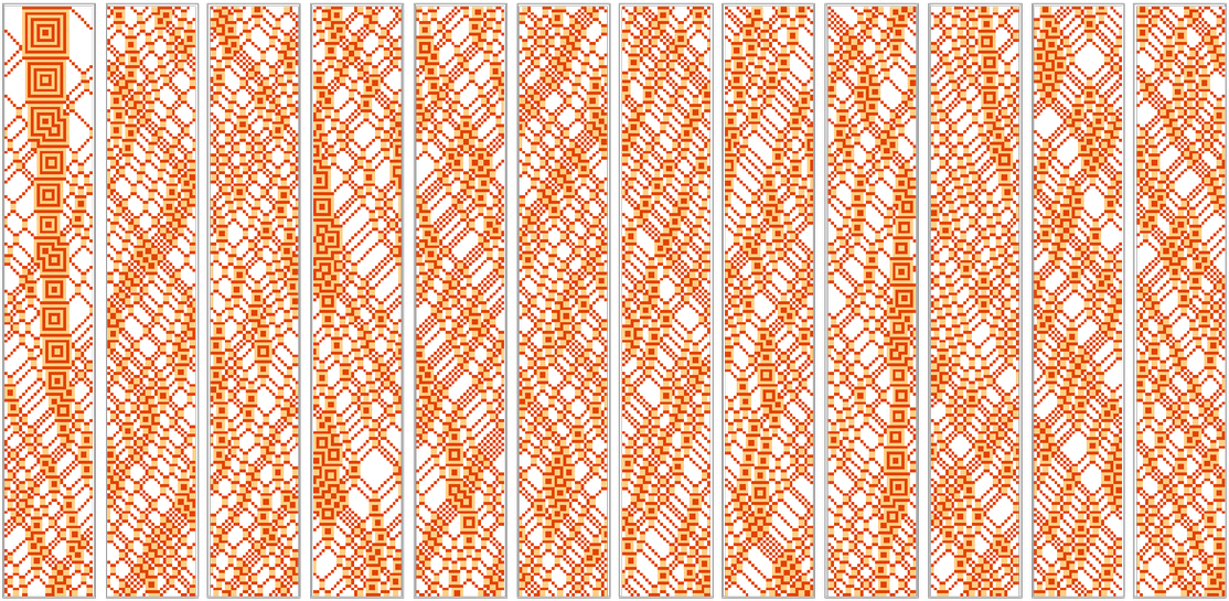
But what about other initial conditions? Here are some samples of what happens:
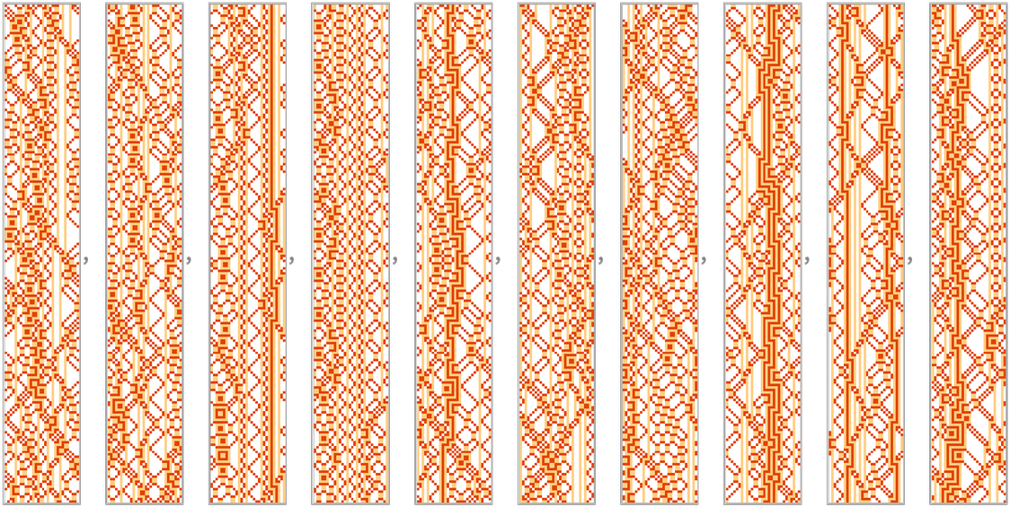
In some cases we again get what appears to be quite random behavior. But in other cases the behavior looks much more structured. Sometimes this is just because there’s a short recurrence time:

And indeed the overall distribution of recurrence times falls off in a first approximation exponentially (though with a definite tail):

But the distribution is quite broad—with a mean of more than 50,000 steps. (The 17-particle initial blob gives a recurrence time of 155,150 steps.) So what happens with “typical” initial conditions that don’t give short recurrences? Here’s an example:

What’s notable here is that unlike for the case of the “simple blob”, there seem to be identifiable traces of the initial conditions that persist for a long time. So what’s going on—and how does it relate to the Second Law?
Given the basic rules for the particle cellular automaton
we immediately know that at least a couple of aspects of the initial conditions will persist forever. In particular, the rules conserve the total number of “particles” (i.e. non-white cells) so that:
![]()
In addition, the number of light or dark cells can change only by increments of 2, and therefore their total number must remain either always even or always odd—and combined with overall particle conservation this then implies that:
![]()
What about other conservation laws? We can formulate the conservation of total particle number as saying that the number of instances of “length-1 blocks” with weights specified as follows is always constant:
Then we can go on and ask about conservation laws associated with longer blocks. For blocks of length 2, there are no new nontrivial conservation laws, though for example the weighted combination of blocks
is nominally “conserved”—but only because it is 0 for any possible configuration.
But in addition to such global conservation laws, there are also more local kinds of regularities. For example, a single “light particle” on its own just stays fixed, and a pair of light particles can always trap a single dark particle between them:

For any separation of light particles, it turns out to always be possible to trap any number of dark particles:
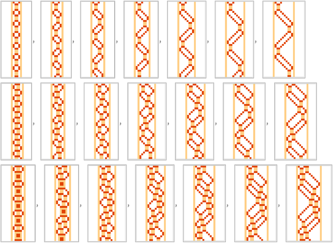
But not every initial configuration of dark particles gets trapped. With separation s and d dark particles, there are a total of Binomial[s,d] possible initial configurations. For d = 2, a fraction
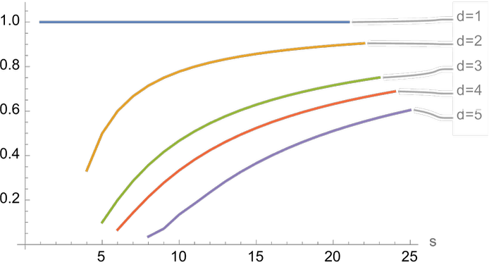
What’s basically going on is that a single dark particle always just “bounces off” a light particle:

But a pair of dark particles can “go through” the light particle, shifting it slightly:

Different things happen with different configurations of dark particles:

And with more complicated “barriers” the behavior can depend in detail on precise phase and separation relationships:

But the basic point is that—although there are various ways they can be modified or destroyed—“light particle walls” can persist for a least a long time. And the result is that if such walls happen to occur in an initial condition they can at least significantly slow down “degradation to randomness”.
For example, this shows evolution over the course of 200,000 steps from a particular initial condition, sampled every 20,000 steps—and even over all these steps we see that there’s definite “wall structure” that survives:
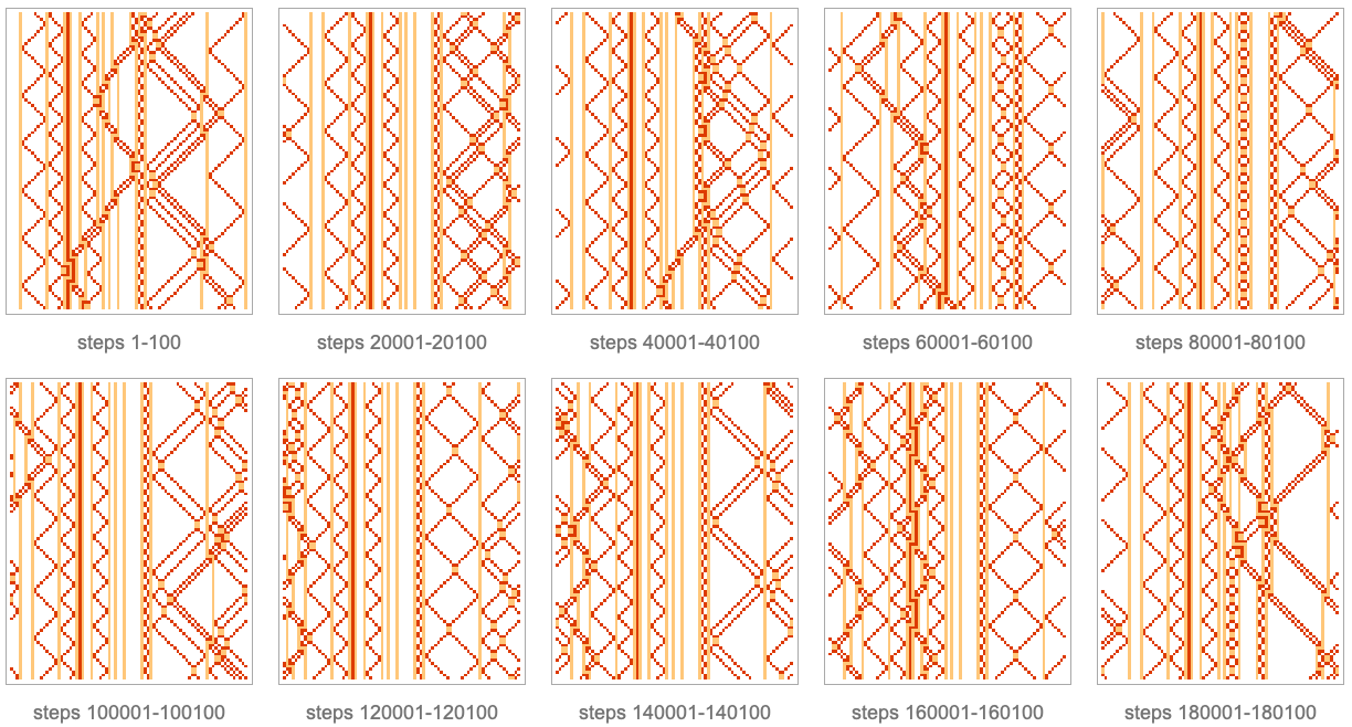
Let’s look at a simpler case: a single light particle surrounded by a few dark particles:

If we plot the position of the light particle we see that for thousands of steps it just jiggles around
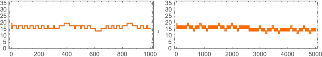
but if one runs it long enough it shows systematic motion at a rate of about 1 position every 1300 steps, wrapping around the cyclic boundary conditions, and eventually returning to its starting point—at the recurrence time of 46,836 steps:

What does all this mean? Essentially the point is that even though something like our particle cellular automaton exhibits computational irreducibility and often generates “featureless” apparent randomness, a system like this is also capable of exhibiting computational reducibility in which traces of the initial conditions can persist, and there isn’t just “generic randomness generation”.
Computational irreducibility is a powerful force. But, as we’ll discuss below, its very presence implies that there must inevitably also be “pockets” of computational reducibility. And once again (as we’ll discuss below) it’s a question of the observer how obvious or not these pockets may be in a particular case, and whether—say for observers like us—they affect what we perceive in terms of the operation of the Second Law.
It’s worth commenting that such issues are not just a feature of systems like our particle cellular automaton. And indeed they’ve appeared—stretching all the way back to the 1950s—pretty much whenever detailed simulations have been done of systems that one might expect would show “Second Law” behavior. The story is typically that, yes, there is apparent randomness generated (though it’s often barely studied as such), just as the Second Law would suggest. But then there’s a big surprise of some kind of unexpected regularity. In arrays of nonlinear springs, there were solitons. In hard-sphere gases, there were “long-time tails”—in which correlations in the motion of spheres were seen to decay not exponentially in time, but rather like power laws.
The phenomenon of long-time tails is actually visible in the cellular automaton “approximation” to hard-sphere gases that we studied above. And its interpretation is a good example of how computational reducibility manifests itself. At a small scale, the motion of our idealized molecules shows computational irreducibility and randomness. But on a larger scale, it’s more like “collective hydrodynamics”, with fluid mechanics effects like vortices. And it’s these much-simpler-to-describe computationally reducible effects that lead to the “unexpected regularities” associated with long-time tails.
When the Second Law Works, and When It Doesn’t
At its core, the Second Law is about evolution from orderly “simple” initial conditions to apparent randomness. And, yes, this is a phenomenon we can certainly see happen in things like hard-sphere gases in which we’re in effect emulating the motion of physical gas molecules. But what about systems with other underlying rules? Because we’re explicitly doing everything computationally, we’re in a position to just enumerate possible rules (i.e. possible programs) and see what they do.
As an example, here are the distinct patterns produced by all 288 3-color reversible block cellular automata that don’t change the all-white state (but don’t necessarily conserve “particle number”):

As is typical to see in the computational universe of simple programs, there’s quite a diversity of behavior. Often we see it “doing the Second Law thing” and “decaying” to apparent randomness

although sometimes taking a while to do so:

But there are also cases where the behavior just stays simple forever

as well as other cases where it takes a fairly long time before it’s clear what’s going to happen:

In many ways, the most surprising thing here is that such simple rules can generate randomness. And as we’ve discussed, that’s in the end what leads to the Second Law. But what about rules that don’t generate randomness, and just produce simple behavior? Well, in these cases the Second Law doesn’t apply.
In standard physics, the Second Law is often applied to gases—and indeed this was its very first application area. But to a solid whose atoms have stayed in more or less fixed positions for a billion years, it really doesn’t usefully apply. And the same is true, say, for a line of masses connected by perfect springs, with perfect linear behavior.
There’s been a quite pervasive assumption that the Second Law is somehow always universally valid. But it’s simply not true. The validity of the Second Law is associated with the phenomenon of computational irreducibility. And, yes, this phenomenon is quite ubiquitous. But there are definitely systems and situations in which it does not occur. And those will not show “Second Law” behavior.
There are plenty of complicated “marginal” cases, however. For example, for a given rule (like the 3 shown here), some initial conditions may not lead to randomness and “Second Law behavior”, while others do:

And as is so often the case in the computational universe there are phenomena one never expects, like the strange “shock-front-like” behavior of the third rule, which produces randomness, but only on a scale determined by the region it’s in:
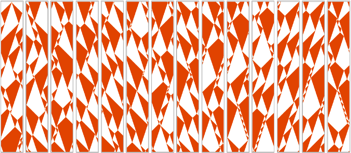
It’s worth mentioning that while restricting to a finite region often yields behavior that more obviously resembles a “box of gas molecules”, the general phenomenon of randomness generation also occurs in infinite regions. And indeed we already know this from the classic example of rule 30. But here it is in a reversible block cellular automaton:

In some simple cases the behavior just repeats, but in other cases it’s nested

albeit sometimes in rather complicated ways:

The Second Law and Order in the Universe
Having identified the computational nature of the core phenomenon of the Second Law we can start to understand in full generality just what the range of this phenomenon is. But what about the ordinary Second Law as it might be applied to familiar physical situations?
Does the ubiquity of computational irreducibility imply that ultimately absolutely everything must “degrade to randomness”? We saw in the previous section that there are underlying rules for which this clearly doesn’t happen. But what about with typical “real-world” systems involving molecules? We’ve seen lots of examples of idealized hard-sphere gases in which we observe randomization. But—as we’ve mentioned several times—even when there’s computational irreducibility, there are always pockets of computational reducibility to be found.
And for example the fact that simple overall gas laws like PV = constant apply to our hard-sphere gas can be viewed as an example of computational reducibility. And as another example, consider a hard-sphere gas in which vortex-like circulation has been set up. To get a sense of what happens we can just look at our simple discrete model. At a microscopic level there’s clearly lots of apparent randomness, and it’s hard to see what’s globally going on:

But if we coarse grain the system by 3×3 blocks of cells with “average velocities” we see that there’s a fairly persistent hydrodynamic-like vortex that can be identified:

Microscopically, there’s computational irreducibility and apparent randomness. But macroscopically the particular form of coarse-grained measurement we’re using picks out a pocket of reducibility—and we see overall behavior whose obvious features don’t show “Second-Law-style” randomness.
And in practice this is how much of the “order” we see in the universe seems to work. At a small scale there’s all sorts of computational irreducibility and randomness. But on a larger scale there are features that we as observers notice that tap into pockets of reducibility, and that show the kind of order that we can describe, for example, with simple mathematical laws.
There’s an extreme version of this in our Physics Project, where the underlying structure of space—like the underlying structure of something like a gas—is full of computational irreducibility, but where there are certain overall features that observers like us notice, and that show computational reducibility. One example involves the large-scale structure of spacetime, as described by general relativity. Another involves the identification of particles that can be considered to “move without change” through the system.
One might have thought—as people often have—that the Second Law would imply a degradation of every feature of a system to uniform randomness. But that’s just not how computational irreducibility works. Because whenever there’s computational irreducibility, there are also inevitably an infinite number of pockets of computational reducibility. (If there weren’t, that very fact could be used to “reduce the irreducibility”.)
And what that means is that when there’s irreducibility and Second-Law-like randomization, there’ll also always be orderly laws to be found. But which of those laws will be evident—or relevant—to a particular observer depends on the nature of that observer.
The Second Law is ultimately a story of the mismatch between the computational irreducibility of underlying systems, and the computational boundedness of observers like us. But the point is that if there’s a pocket of computational reducibility that happens to be “a fit” for us as observers, then despite our computational limitations, we’ll be perfectly able to recognize the orderliness that’s associated with it—and we won’t think that the system we’re looking at has just “degraded to randomness”.
So what this means is that there’s ultimately no conflict between the existence of order in the universe, and the operation of the Second Law. Yes, there’s an “ocean of randomness” generated by computational irreducibility. But there’s also inevitably order that lives in pockets of reducibility. And the question is just whether a particular observer “notices” a given pocket of reducibility, or whether they only “see” the “background” of computational irreducibility.
In the “hydrodynamics” example above, the “observer” picks out a “slice” of behavior by looking at aggregated local averages. But another way for an observer to pick out a “slice” of behavior is just to look only at a specific region in a system. And in that case one can observe simpler behavior because in effect “the complexity has radiated away”. For example, here are reversible cellular automata where a random initial block is “simplified” by “radiating its information out”:
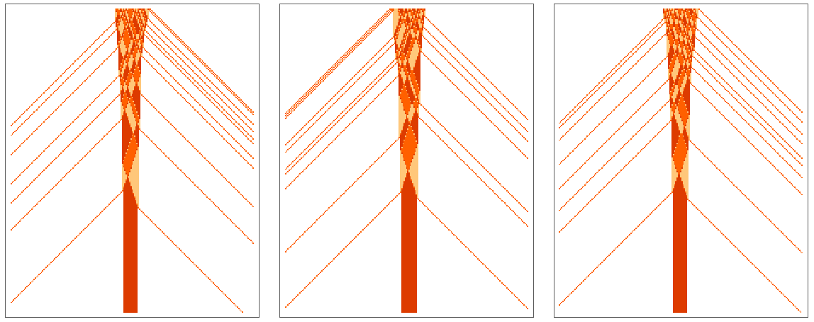

If one picked up all those “pieces of radiation” one would be able—with appropriate computational effort—to reconstruct all the randomness in the initial condition. But if we as observers just “ignore the radiation to infinity” then we’ll again conclude that the system has evolved to a simpler state—against the “Second-Law trend” of increasing randomness.
Class 4 and the Mechanoidal Phase
When I first studied cellular automata back in the 1980s, I identified four basic classes of behavior that are seen when starting from generic initial conditions—as exemplified by:
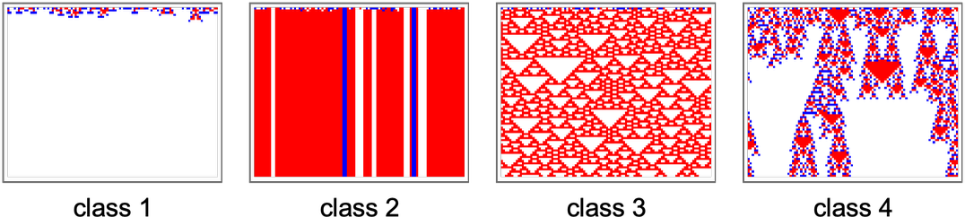
Class 1 essentially always evolves to the same final “fixed-point” state, immediately destroying information about its initial state. Class 2, however, works a bit like solid matter, essentially just maintaining whatever configuration it was started in. Class 3 works more like a gas or a liquid, continually “mixing things up” in a way that looks quite random. But class 4 does something more complicated.
In class 3 there aren’t significant identifiable persistent structures, and everything always seems to quickly get randomized. But the distinguishing feature of class 4 is the presence of identifiable persistent structures, whose interactions effectively define the activity of the system.
So how do these types of behavior relate to the Second Law? Class 1 involves intrinsic irreversibility, and so doesn’t immediately connect to standard Second Law behavior. Class 2 is basically too static to follow the Second Law. But class 3 shows quintessential Second Law behavior, with rapid evolution to “typical random states”. And it’s class 3 that captures the kind of behavior that’s seen in typical Second Law systems, like gases.
But what about class 4? Well, it’s a more complicated story. The “level of activity” in class 4—while above class 2—is in a sense below class 3. But unlike in class 3, where there is typically “too much activity” to “see what’s going on”, class 4 often gives one the idea that it’s operating in a “more potentially understandable” way. There are many different detailed kinds of behavior that appear in class 4 systems. But here are a few examples in reversible block cellular automata:
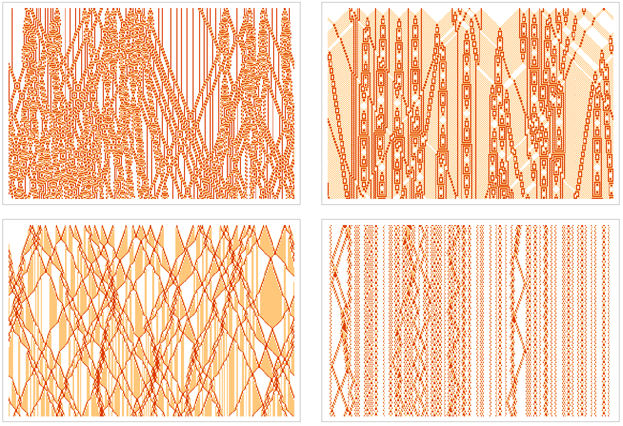
Looking at the first rule, it’s easy to identify some simple persistent structures, some stationary, some moving:
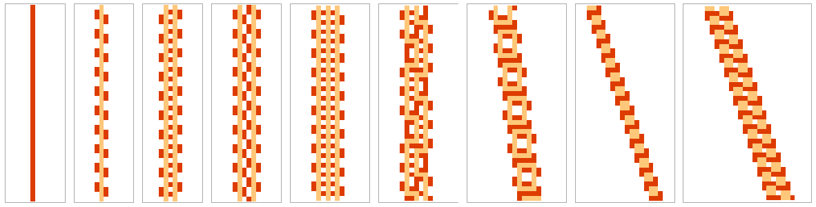
But even with this rule, many other things can happen too

and in the end the whole behavior of the system is built up from combinations and interactions of structures like these.
The second rule above behaves in an immediately more elaborate way. Here it is starting from a random initial condition:

Starting just from ![]() one gets:
one gets:

Sometimes the behavior seems simpler

though even in the last case here, there is elaborate “number-theoretical” behavior that seems to never quite become either periodic or nested:

We can think of any cellular automaton—or any system based on rules—as “doing a computation” when it evolves. Class 1 and 2 systems basically behave in computationally simple ways. But as soon as we reach class 3 we’re dealing with computational irreducibility, and with a “density of computation” that lets us decode almost nothing about what comes out, with the result that what we see we can basically describe only as “apparently random”. Class 4 no doubt has the same ultimate computational irreducibility—and the same ultimate computational capabilities—as class 3. But now the computation is “less dense”, and seemingly more accessible to human interpretation. In class 3 it’s difficult to imagine making any kind of “symbolic summary” of what’s going on. But in class 4, we see definite structures whose behavior we can imagine being able to describe in a symbolic way, building up what we can think of as a “human-accessible narrative” in which we talk about “structure X collides with structure Y to produce structure Z” and so on.
And indeed if we look at the picture above, it’s not too difficult to imagine that it might correspond to the execution trace of a computation we might do. And more than that, given the “identifiable components” that arise in class 4 systems, one can imagine assembling these to explicitly set up particular computations one wants to do. In a class 3 system “randomness” always just “spurts out”, and one has very little ability to “meaningfully control” what happens. But in a class 4 system, one can potentially do what amounts to traditional engineering or programming to set up an arrangement of identifiable component “primitives” that achieves some particular purpose one has chosen.
And indeed in a case like the rule 110 cellular automaton we know that it’s possible to perform any computation in this way, proving that the system is capable of universal computation, and providing a piece of evidence for the phenomenon of computational irreducibility. No doubt rule 30 is also computation universal. But the point is that with our current ways of analyzing things, class 3 systems like this don’t make this something we can readily recognize.
Like so many other things we’re discussing, this is basically again a story of observers and their capabilities. If observers like us—with our computational boundedness—are going to be able to “get things into our minds” we seem to need to break them down to the point where they can be described in terms of modest numbers of types of somewhat-independent parts. And that’s what the “decomposition into identifiable structures” that we observe in class 4 systems gives us the opportunity to do.
What about class 3? Notwithstanding things like our discussion of traces of initial conditions above, our current powers of perception just don’t seem to let us “understand what’s going on” to the point where we can say much more than there’s apparent randomness. And of course it’s this very point that we’re arguing is the basis for the Second Law. Could there be observers who could “decode class 3 systems”? In principle, absolutely yes. And even if the observers—like us—are computationally bounded, we can expect that there will be at least some pockets of computational reducibility that could be found that would allow progress to be made.
But as of now—with the methods of perception and analysis currently at our disposal—there’s something very different for us about class 3 and class 4. Class 3 shows quintessential “apparently random” behavior, like molecules in a gas. Class 4 shows behavior that looks more like the “insides of a machine” that could have been “intentionally engineered for a purpose”. Having a system that is like this “in bulk” is not something familiar, say from physics. There are solids, and liquids, and gases, whose components have different general organizational characteristics. But what we see in class 4 is something yet different—and quite unfamiliar.
Like solids, liquids and gases, it’s something that can exist “in bulk”, with any number of components. We can think of it as a “phase” of a system. But it’s a new type of phase, that we might call a “mechanoidal phase”.
How do we recognize this phase? Again, it’s a question of the observer. Something like a solid phase is easy for observers like us to recognize. But even the distinction between a liquid and a gas can be more difficult to recognize. And to recognize the mechanoidal phase we basically have to be asking something like “Is this a computation we recognize?”
How does all this relate to the Second Law? Class 3 systems—like gases—immediately show typical “Second Law” behavior, characterized by randomness, entropy increase, equilibrium, and so on. But class 4 systems work differently. They have new characteristics that don’t fit neatly into the rubric of the Second Law.
No doubt one day we will have theories of the mechanoidal phase just like today we have theories of gases, of liquids and of solids. Likely those theories will have to get more sophisticated in characterizing the observer, and in describing what kinds of coarse graining can reasonably be done. Presumably there will be some kind of analog of the Second Law that leverages the difference between the capabilities and features of the observer and the system they’re observing. But in the mechanoidal phase there is in a sense less distance between the mechanism of the system and the mechanism of the observer, so we probably can’t expect a statement as ultimately simple and clear-cut as the usual Second Law.
The Mechanoidal Phase and Bulk Molecular Biology
The Second Law has long had an uneasy relationship with biology. “Physical” systems like gases readily show the “decay” to randomness expected from the Second Law. But living systems instead somehow seem to maintain all sorts of elaborate organization that doesn’t immediately “decay to randomness”— and indeed actually seems able to grow just through “processes of biology”.
It’s easy to point to the continual absorption of energy and material by living systems—as well as their eventual death and decay—as reasons why such systems might still at least nominally follow the Second Law. But even if at some level this works, it’s not particularly useful in letting us talk about the actual significant “bulk” features of living systems—in the kind of way that the Second Law routinely lets us make “bulk” statements about things like gases.
So how might we begin to describe living systems “in bulk”? I suspect a key is to think of them as being in large part in what we’re here calling the mechanoidal phase. If one looks inside a living organism at a molecular scale, there are some parts that can reasonably be described as solid, liquid or gas. But what molecular biology has increasingly shown is that there’s often much more elaborate molecular-scale organization than exist in those phases—and moreover that at least at some level this organization seems “describable” and “machine-like”, with molecules and collections of molecules that we can say have “particular functions”, often being “carefully” and actively transported by things like the cytoskeleton.
In any given organism, there are for example specific proteins defined by the genomics of the organism, that behave in specific ways. But one suspects that there’s also a higher-level or “bulk” description that allows one to make at least some kinds of general statements. There are already some known general principles in biology—like the concept of natural selection, or the self-replicating digital character of genetic information—that let one come to various conclusions independent of microscopic details.
And, yes, in some situations the Second Law provides certain kinds of statements about biology. But I suspect that there are much more powerful and significant principles to be discovered, that in fact have the potential to unlock a whole new level of global understanding of biological systems and processes.
It’s perhaps worth mentioning an analogy in technology. In a microprocessor what we can think of as the “working fluid” is essentially a gas of electrons. At some level the Second Law has things to say about this gas of electrons, for example describing scattering processes that lead to electrical resistance. But the vast majority of what matters in the behavior of this particular gas of electrons is defined not by things like this, but by the elaborate pattern of wires and switches that exist in the microprocessor, and that guide the motion of the electrons.
In living systems one sometimes also cares about the transport of electrons—though more often it’s atoms and ions and molecules. And living systems often seem to provide what one can think of as a close analog of wires for transporting such things. But what is the arrangement of these “wires”? Ultimately it’ll be defined by the application of rules derived from things like the genome of the organism. Sometimes the results will for example be analogous to crystalline or amorphous solids. But in other cases one suspects that it’ll be better described by something like the mechanoidal phase.
Quite possibly this may also provide a good bulk description of technological systems like microprocessors or large software codebases. And potentially then one might be able to have high-level laws—analogous to the Second Law—that would make high-level statements about these technological systems.
It’s worth mentioning that a key feature of the mechanoidal phase is that detailed dynamics—and the causal relations it defines—matter. In something like a gas it’s perfectly fine for most purposes to assume “molecular chaos”, and to say that molecules are arbitrarily mixed. But the mechanoidal phase depends on the “detailed choreography” of elements. It’s still a “bulk phase” with arbitrarily many elements. But things like the detailed history of interactions of each individual element matter.
In thinking about typical chemistry—say in a liquid or gas phase—one’s usually just concerned with overall concentrations of different kinds of molecules. In effect one assumes that the “Second Law has acted”, and that everything is “mixed randomly” and the causal histories of molecules don’t matter. But it’s increasingly clear that this picture isn’t correct for molecular biology, with all its detailed molecular-scale structures and mechanisms. And instead it seems more promising to model what’s there as being in the mechanoidal phase.
So how does this relate to the Second Law? As we’ve discussed, the Second Law is ultimately a reflection of the interplay between underlying computational irreducibility and the limited computational capabilities of observers like us. But within computational irreducibility there are inevitably always “pockets” of computational reducibility—which the observer may or may not care about, or be able to leverage.
In the mechanoidal phase there is ultimately computational irreducibility. But a defining feature of this phase is the presence of “local computational reducibility” visible in the existence of identifiable localized structures. Or, in other words, even to observers like us, it’s clear that the mechanoidal phase isn’t “uniformly computationally irreducible”. But just what general statements can be made about it will depend—potentially in some detail—on the characteristics of the observer.
We’ve managed to get a long way in discussing the Second Law—and even more so in doing our Physics Project—by making only very basic assumptions about observers. But to be able to make general statements about the mechanoidal phase—and living systems—we’re likely to have to say more about observers. If one’s presented with a lump of biological tissue one might at first just describe it as some kind of gel. But we know there’s much more to it. And the question is what features we can perceive. Right now we can see with microscopes all kinds of elaborate spatial structures. Perhaps in the future there’ll be technology that also lets us systematically detect dynamic and causal structures. And it’ll be the interplay of what we perceive with what’s computationally going on underneath that’ll define what general laws we will be able to see emerge.
We already know we won’t just get the ordinary Second Law. But just what we will get isn’t clear. But somehow—perhaps in several variants associated with different kinds of observers—what we’ll get will be something like “general laws of biology”, much like in our Physics Project we get general laws of spacetime and of quantum mechanics, and in our analysis of metamathematics we get “general laws of mathematics”.
The Thermodynamics of Spacetime
Traditional twentieth-century physics treats spacetime a bit like a continuous fluid, with its characteristics being defined by the continuum equations of general relativity. Attempts to align this with quantum field theory led to the idea of attributing an entropy to black holes, in essence to represent the number of quantum states “hidden” by the event horizon of the black hole. But in our Physics Project there is a much more direct way of thinking about spacetime in what amount to thermodynamic terms.
A key idea of our Physics Project is that there’s something “below” the “fluid” representation of spacetime—and in particular that space is ultimately made of discrete elements, whose relations (which can conveniently be represented by a hypergraph) ultimately define everything about the structure of space. This structure evolves according to rules that are somewhat analogous to those for block cellular automata, except that now one is doing replacements not for blocks of cell values, but instead for local pieces of the hypergraph.
So what happens in a system like this? Sometimes the behavior is simple. But very often—much like in many cellular automata—there is great complexity in the structure that develops even from simple initial conditions:

It’s again a story of computational irreducibility, and of the generation of apparent randomness. The notion of “randomness” is a bit less straightforward for hypergraphs than for arrays of cell values. But what ultimately matters is what “observers like us” perceive in the system. A typical approach is to look at geodesic balls that encompass all elements within a certain graph distance of a given element—and then to study the effective geometry that emerges in the large-scale limit. It’s then a bit like seeing fluid dynamics emerge from small-scale molecular dynamics, except that here (after navigating many technical issues) it’s the Einstein equations of general relativity that emerge.
But the fact that this can work relies on something analogous to the Second Law. It has to be the case that the evolution of the hypergraph leads at least locally to something that can be viewed as “uniformly random”, and on which statistical averages can be done. In effect, the microscopic structure of spacetime is reaching some kind of “equilibrium state”, whose detailed internal configuration “seems random”—but which has definite “bulk” properties that are perceived by observers like us, and give us the impression of continuous spacetime.
As we’ve discussed above, the phenomenon of computational irreducibility means that apparent randomness can arise completely deterministically just by following simple rules from simple initial conditions. And this is presumably what basically happens in the evolution and “formation” of spacetime. (There are some additional complications associated with multicomputation that we’ll discuss at least to some extent later.)
But just like for the systems like gases that we’ve discussed above, we can now start talking directly about things like entropy for spacetime. As “large-scale observers” of spacetime we’re always effectively doing coarse graining. So now we can ask how many microscopic configurations of spacetime (or space) are consistent with whatever result we get from that coarse graining.
As a toy example, consider just enumerating all possible graphs (say up to a given size), then asking which of them have a certain pattern of volumes for geodesic balls (i.e. a certain sequence of numbers of distinct nodes within a given graph distance of a particular node). The “coarse-grained entropy” is simply determined by the number of graphs in which the geodesic ball volumes start in the same way. Here are all trivalent graphs (with up to 24 nodes) that have various such geodesic ball “signatures” (most, but not all, turn out to be vertex transitive; these graphs were found by filtering a total of 125,816,453 possibilities):
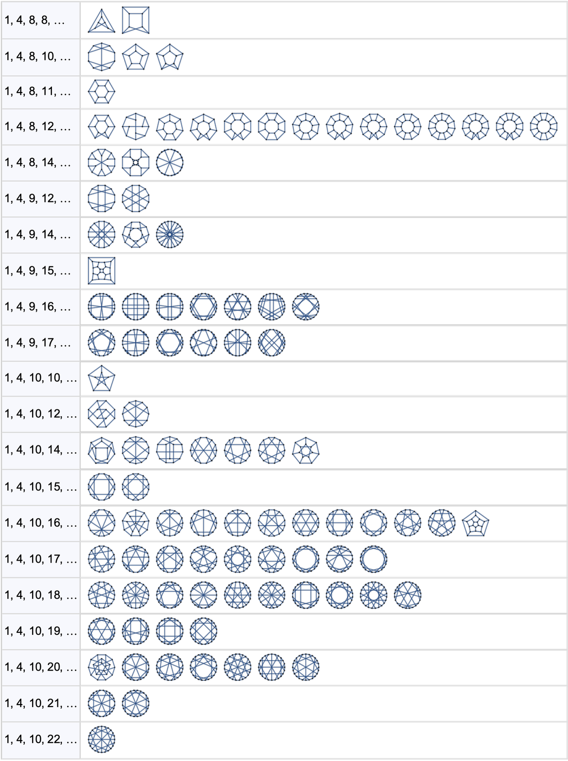
We can think of the different numbers of graphs in each case as representing different entropies for a tiny fragment of space constrained to have a given “coarse-grained” structure. At the graph sizes we’re dealing with here, we’re very far from having a good approximation to continuum space. But assume we could look at much larger graphs. Then we might ask how the entropy varies with “limiting geodesic ball signature”—which in the continuum limit is determined by dimension, curvature, etc.
For a general “disembodied lump of spacetime” this is all somewhat hard to define, particularly because it depends greatly on issues of “gauge” or of how the spacetime is foliated into spacelike slices. But event horizons, being in a sense much more global, don’t have such issues, and so we can expect to have fairly invariant definitions of spacetime entropy in this case. And the expectation would then be that for example the entropy we would compute would agree with the “standard” entropy computed for example by analyzing quantum fields or strings near a black hole. But with the setup we have here we should also be able to ask more general questions about spacetime entropy—for example seeing how it varies with features of arbitrary gravitational fields.
In most situations the spacetime entropy associated with any spacetime configuration that we can successfully identify at our coarse-grained level will be very large. But if we could ever find a case where it is instead small, this would be somewhere we could expect to start seeing a breakdown of the continuum “equilibrium” structure of spacetime, and where evidence of discreteness should start to show up.
We’ve so far mostly been discussing hypergraphs that represent instantaneous states of space. But in talking about spacetime we really need to consider causal graphs that map out the causal relationships between updating events in the hypergraph, and that represent the structure of spacetime. And once again, such graphs can show apparent randomness associated with computational irreducibility.
One can make causal graphs for all sorts of systems. Here is one for a “Newton’s cradle” configuration of an (effectively 1D) hard-sphere gas, in which events are collisions between spheres, and two events are causally connected if a sphere goes from one to the other:
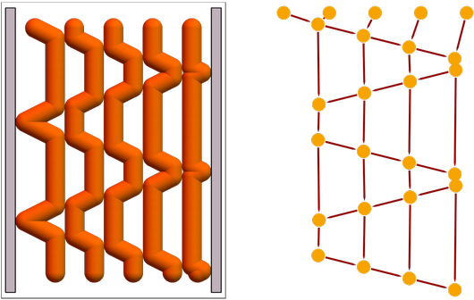
And here is an example for a 2D hard-sphere case, with the causal graph now reflecting the generation of apparently random behavior:
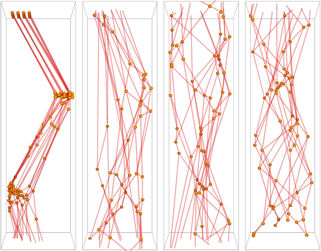
Similar to this, we can make a causal graph for our particle cellular automaton, in which we consider it an event whenever a block changes (but ignore “no-change updates”):

For spacetime, features of the causal graph have some definite interpretations. We define the reference frame we’re using by specifying a foliation of the causal graph. And one of the results of our Physics Project is then that the flux of causal edges through the spacelike hypersurfaces our foliation defines can be interpreted directly as the density of physical energy. (The flux through timelike hypersurfaces gives momentum.)
One can make a surprisingly close analogy to causal graphs for hard-sphere gases—except that in a hard-sphere gas the causal edges correspond to actual, nonrelativistic motion of idealized molecules, while in our model of spacetime the causal edges are abstract connections that are in effect always lightlike (i.e. they correspond to motion at the speed of light). In both cases, reducing the number of events is like reducing some version of temperature—and if one approaches no-event “absolute zero” both the gas and spacetime will lose their cohesion, and no longer allow propagation of effects from one part of the system to another.
If one increases density in the hard-sphere gas one will eventually form something like a solid, and in this case there will be a regular arrangement of both spheres and the causal edges. In spacetime something similar may happen in connection with event horizons—which may behave like an “ordered phase” with causal edges aligned.
What happens if one combines thinking about spacetime and thinking about matter? A long-unresolved issue concerns systems with many gravitationally attracting bodies—say a “gas” of stars or galaxies. While the molecules in an ordinary gas might evolve to an apparently random configuration in a standard “Second Law way”, gravitationally attracting bodies tend to clump together to make what seem like “progressively simpler” configurations.
It could be that this is a case where the standard Second Law just doesn’t apply, but there’s long been a suspicion that the Second Law can somehow be “saved” by appropriately associating an entropy with the structure of spacetime. In our Physics Project, as we’ve discussed, there’s always entropy associated with our coarse-grained perception of spacetime. And it’s conceivable that, at least in terms of overall counting of states, increased “organization” of matter could be more than balanced by enlargement in the number of available states for spacetime.
We’ve discussed at length above the idea that “Second Law behavior” is the result of us as observers (and preparers of initial states) being “computationally weak” relative to the computational irreducibility of the underlying dynamics of systems. And we can expect that very much the same thing will happen for spacetime. But what if we could make a Maxwell’s demon for spacetime? What would this mean?
One rather bizarre possibility is that it could allow faster-than-light “travel”. Here’s a rough analogy. Gas molecules—say in air in a room—move at roughly the speed of sound. But they’re always colliding with other molecules, and getting their directions randomized. But what if we had a Maxwell’s-demon-like device that could tell us at every collision which molecule to ride on? With an appropriate choice for the sequence of molecules we could then potentially “surf” across the room at roughly the speed of sound. Of course, to have the device work it’d have to overcome the computational irreducibility of the basic dynamics of the gas.
In spacetime, the causal graph gives us a map of what event can affect what other event. And insofar as we just treat spacetime as “being in uniform equilibrium” there’ll be a simple correspondence between “causal distance” and what we consider distance in physical space. But if we look down at the level of individual causal edges it’ll be more complicated. And in general we could imagine that an appropriate “demon” could predict the microscopic causal structure of spacetime, and carefully pick causal edges that could “line up” to “go further in space” than the “equilibrium expectation”.
Of course, even if this worked, there’s still the question of what could be “transported” through such a “tunnel”—and for example even a particle (like an electron) presumably involves a vast number of causal edges, that one wouldn’t be able to systematically organize to fit through the tunnel. But it’s interesting to realize that in our Physics Project the idea that “nothing can go faster than light” becomes something very much analogous to the Second Law: not a fundamental statement about underlying rules, but rather a statement about our interaction with them, and our capabilities as observers.
So if there’s something like the Second Law that leads to the structure of spacetime as we typically perceive it, what can be said about typical issues in thermodynamics in connection with spacetime? For example, what’s the story with perpetual motion machines in spacetime?
Even before talking about the Second Law, there are already issues with the First Law of thermodynamics—because in a cosmological setting there isn’t local conservation of energy as such, and for example the expansion of the universe can transfer energy to things. But what about the Second Law question of “getting mechanical work from heat”? Presumably the analog of “mechanical work” is a gravitational field that is “sufficiently organized” that observers like us can readily detect it, say by seeing it pull objects in definite directions. And presumably a perpetual motion machine based on violating the Second Law would then have to take the heat-like randomness in “ordinary spacetime” and somehow organize it into a systematic and measurable gravitational field. Or, in other words, “perpetual motion” would somehow have to involve a gravitational field “spontaneously being generated” from the microscopic structure of spacetime.
Just like in ordinary thermodynamics, the impossibility of doing this involves an interplay between the observer and the underlying system. And conceivably it might be possible that there could be an observer who can measure specific features of spacetime that correspond to some slice of computational reducibility in the underlying dynamics—say some weird configuration of “spontaneous motion” of objects. But absent this, a “Second-Law-violating” perpetual motion machine will be impossible.
Quantum Mechanics
Like statistical mechanics (and thermodynamics), quantum mechanics is usually thought of as a statistical theory. But whereas the statistical character of statistical mechanics one imagines to come from a definite, knowable “mechanism underneath”, the statistical character of quantum mechanics has usually just been treated as a formal, underivable “fact of physics”.
In our Physics Project, however, the story is different, and there’s a whole lower-level structure—ultimately rooted in the ruliad—from which quantum mechanics and its statistical character appears to be derived. And, as we’ll discuss, that derivation in the end has close connections both to what we’ve said about the standard Second Law, and to what we’ve said about the thermodynamics of spacetime.
In our Physics Project the starting point for quantum mechanics is the unavoidable fact that when one’s applying rules to transform hypergraphs, there’s typically more than one rewrite that can be done to any given hypergraph. And the result of this is that there are many different possible “paths of history” for the universe.
As a simple analog, consider rewriting not hypergraphs but strings. And doing this, we get for example:

This is a deterministic representation of all possible “paths of history”, but in a sense it’s very wasteful, among other things because it includes multiple copies of identical strings (like BBBB). If we merge such identical copies, we get what we call a multiway graph, that contains both branchings and mergings:

In the “innards” of quantum mechanics one can imagine that all these paths are being followed. So how is it that we as observers perceive definite things to happen in the world? Ultimately it’s a story of coarse graining, and of us conflating different paths in the multiway graph.
But there’s a wrinkle here. In statistical mechanics we imagine that we can observe from outside the system, implementing our coarse graining by sampling particular features of the system. But in quantum mechanics we imagine that the multiway system describes the whole universe, including us. So then we have the peculiar situation that just as the universe is branching and merging, so too are our brains. And ultimately what we observe is therefore the result of a branching brain perceiving a branching universe.
But given all those branches, can we just decide to conflate them into a single thread of experience? In a sense this is a typical question of coarse graining and of what we can consistently equivalence together. But there’s something a bit different here because without the “coarse graining” we can’t talk at all about “what happened”, only about what might be happening. Put another way, we’re now fundamentally dealing not with computation (like in a cellular automaton) but with multicomputation.
And in multicomputation, there are always two fundamental kinds of operations: the generation of new states from old, and the equivalencing of states, effectively by the observer. In ordinary computation, there can be computational irreducibility in the process of generating a thread of successive states. In multicomputation, there can be multicomputational irreducibility in which in a sense all computations in the multiway system have to be done in order even to determine a single equivalenced result. Or, put another way, you can’t shortcut following all the paths of history. If you try to equivalence at the beginning, the equivalence class you’ve built will inevitably be “shredded” by the evolution, forcing you to follow each path separately.
It’s worth commenting that just as in classical mechanics, the “underlying dynamics” in our description of quantum mechanics are reversible. In the original unmerged evolution tree above, we could just reverse each rule and from any point uniquely construct a “backwards tree”. But once we start merging and equivalencing, there isn’t the same kind of “direct reversibility”—though we can still count possible paths to determine that we preserve “total probability”.
In ordinary computational systems, computational irreducibility implies that even from simple initial conditions we can get behavior that “seems random” with respect to most computationally bounded observations. And something directly analogous happens in multicomputational systems. From simple initial conditions, we generate collections of paths of history that “seem random” with respect to computationally bounded equivalencing operations, or, in other words, to observers who do computationally bounded coarse graining of different paths of history.
When we look at the graphs we’ve drawn representing the evolution of a multiway system, we can think of there being a time direction that goes down the page, following the arrows that point from states to their successors. But across the page, in the transverse direction, we can think of there as being a space in which different paths of history are laid—what we call “branchial space”.
A typical way to start constructing branchial space is to take slices across the multiway graph, then to form a branchial graph in which two states are joined if they have a common ancestor on the step before (which means we can consider them “entangled”):
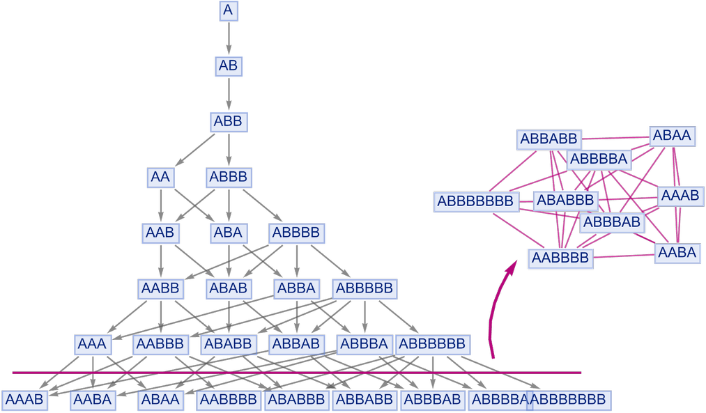
Although the details remain to be clarified, it seems as if in the standard formalism of quantum mechanics, distance in branchial space corresponds essentially to quantum phase, so that, for example, particles whose phases would make them show destructive interference will be at “opposite ends” of branchial space.
So how do observers relate to branchial space? Basically what an observer is doing is to coarse grain in branchial space, equivalencing certain paths of history. And just as we have a certain extent in physical space, which determines our coarse graining of gases, and—at a much smaller scale—of the structure of spacetime, so also we have an extent in branchial space that determines our coarse graining across branches of history.
But this is where multicomputational irreducibility and the analog of the Second Law are crucial. Because just as we imagine that gases—and spacetime—achieve a certain kind of “unique random equilibrium” that leads us to be able to make consistent measurements of them, so also we can imagine that in quantum mechanics there is in effect a “branchial space equilibrium” that is achieved.
Think of a box of gas in equilibrium. Put two pistons on different sides of the box. So long as they don’t perturb the gas too much, they’ll both record the same pressure. And in our Physics Project it’s the same story with observers and quantum mechanics. Most of the time there’ll be enough effective randomness generated by the multicomputationally irreducible evolution of the system (which is completely deterministic at the level of the multiway graph) that a computationally bounded observer will always see the same “equilibrium values”.
A central feature of quantum mechanics is that by making sufficiently careful measurements one can see what appear to be random results. But where does that randomness come from? In the usual formalism for quantum mechanics, the idea of purely probabilistic results is just burnt into the formal structure. But in our Physics Project, the apparent randomness one sees has a definite, “mechanistic” origin. And it’s basically the same as the origin of randomness for the standard Second Law, except that now we’re dealing with multicomputational rather than pure computational irreducibility.
By the way, the “Bell’s inequality” statement that quantum mechanics cannot be based on “mechanistic randomness” unless it comes from a nonlocal theory remains true in our Physics Project. But in the Physics Project we have an immediate ubiquitous source of “nonlocality”: the equivalencing or coarse graining “across” branchial space done by observers.
(We’re not discussing the role of physical space here. But suffice it to say that instead of having each node of the multiway graph represent a complete state of the universe, we can make an extended multiway graph in which different spatial elements—like different paths of history—are separated, with their “causal entanglements” then defining the actual structure of space, in a spatial analog of the branchial graph.)
As we’ve already noted, the complete multiway graph is entirely deterministic. And indeed if we have a complete branchial slice of the graph, this can be used to determine the whole future of the graph (the analog of “unitary evolution” in the standard formalism of quantum mechanics). But if we equivalence states—corresponding to “doing a measurement”—then we won’t have enough information to uniquely determine the future of the system, at least when it comes to what we consider to be quantum effects.
At the outset, we might have thought that statistical mechanics, spacetime mechanics and quantum mechanics were all very different theories. But what our Physics Project suggests is that in fact they are all based on a common, fundamentally computational phenomenon.
So what about other ideas associated with the standard Second Law? How do they work in the quantum case?
Entropy, for example, now just becomes a measure of the number of possible configurations of a branchial graph consistent with a certain coarse-grained measurement. Two independent systems will have disconnected branchial graphs. But as soon as the systems interact, their branchial graphs will connect, and the number of possible graph configurations will change, leading to an “entanglement entropy”.
One question about the quantum analog of the Second Law is what might correspond to “mechanical work”. There may very well be highly structured branchial graphs—conceivably associated with things like coherent states—but it isn’t yet clear how they work and whether existing kinds of measurements can readily detect them. But one can expect that multicomputational irreducibility will tend to produce branchial graphs that can’t be “decoded” by most computationally bounded measurements—so that, for example, “quantum perpetual motion”, in which “branchial organization” is spontaneously produced, can’t happen.
And in the end randomness in quantum measurements is happening for essentially the same basic reason we’d see randomness if we looked at small numbers of molecules in a gas: it’s not that there’s anything fundamentally not deterministic underneath, it’s just there’s a computational process that’s making things too complicated for us to “decode”, at least as observers with bounded computational capabilities. In the case of the gas, though, we’re sampling molecules at different places in physical space. But in quantum mechanics we’re doing the slightly more abstract thing of sampling states of the system at different places in branchial space. But the same fundamental randomization is happening, though now through multicomputational irreducibility operating in branchial space.
The Future of the Second Law
The original formulation of the Second Law a century and a half ago—before even the existence of molecules was established—was an impressive achievement. And one might assume that over the course of 150 years—with all the mathematics and physics that’s been done—a complete foundational understanding of the Second Law would long ago have been developed. But in fact it has not. And from what we’ve discussed here we can now see why. It’s because the Second Law is ultimately a computational phenomenon, and to understand it requires an understanding of the computational paradigm that’s only very recently emerged.
Once one starts doing actual computational experiments in the computational universe (as I already did in the early 1980s) the core phenomenon of the Second Law is surprisingly obvious—even if it violates one’s traditional intuition about how things should work. But in the end, as we have discussed here, the Second Law is a reflection of a very general, if deeply computational, idea: an interplay between computational irreducibility and the computational limitations of observers like us. The Principle of Computational Equivalence tells us that computational irreducibility is inevitable. But the limitation of observers is something different: it’s a kind of epiprinciple of science that’s in effect a formalization of our human experience and our way of doing science.
Can we tighten up the formulation of all this? Undoubtedly. We have various standard models of the computational process—like Turing machines and cellular automata. We still need to develop an “observer theory” that provides standard models for what observers like us can do. And the more we can develop such a theory, the more we can expect to make explicit proofs of specific statements about the Second Law. Ultimately these proofs will have solid foundations in the Principle of Computational Equivalence (although there remains much to formalize there too), but will rely on models for what “observers like us” can be like.
So how general do we expect the Second Law to be in the end? In the past couple of sections we’ve seen that the core of the Second Law extends to spacetime and to quantum mechanics. But even when it comes to the standard subject matter of statistical mechanics, we expect limitations and exceptions to the Second Law.
Computational irreducibility and the Principle of Computational Equivalence are very general, but not very specific. They talk about the overall computational sophistication of systems and processes. But they do not say that there are no simplifying features. And indeed we expect that in any system that shows computational irreducibility, there will always be arbitrarily many “slices of computational reducibility” that can be found.
The question then is whether those slices of reducibility will be what an observer can perceive, or will care about. If they are, then one won’t see Second Law behavior. If they’re not, one will just see “generic computational irreducibility” and Second Law behavior.
How can one find the slices of reducibility? Well, in general that’s irreducibly hard. Every slice of reducibility is in a sense a new scientific or mathematical principle. And the computational irreducibility involved in finding such reducible slices basically speaks to the ultimately unbounded character of the scientific and mathematical enterprise. But once again, even though there might be an infinite number of slices of reducibility, we still have to ask which ones matter to us as observers.
The answer could be one thing for studying gases, and another, for example, for studying molecular biology, or social dynamics. The question of whether we’ll see “Second Law behavior” then boils to whether whatever we’re studying turns out to be something that doesn’t simplify, and ends up showing computational irreducibility.
If we have a sufficiently small system—with few enough components—then the computational irreducibility may not be “strong enough” to stop us from “going beyond the Second Law”, and for example constructing a successful Maxwell’s demon. And indeed as computer and sensor technology improve, it’s becoming increasingly feasible to do measurement and set up control systems that effectively avoid the Second Law in particular, small systems.
But in general the future of the Second Law and its applicability is really all about how the capabilities of observers develop. What will future technology, and future paradigms, do to our ability to pick away at computational irreducibility?
In the context of the ruliad, we are currently localized in rulial space based on our existing capabilities. But as we develop further we are in effect “colonizing” rulial space. And a system that may look random—and may seem to follow the Second Law—from one place in rulial space may be “revealed as simple” from another.
There is an issue, though. Because the more we as observers spread out in rulial space, the less coherent our experience will become. In effect we’ll be following a larger bundle of threads in rulial space, which makes who “we” are less definite. And in the limit we’ll presumably be able to encompass all slices of computational reducibility, but at the cost of having our experience “incoherently spread” across all of them.
It’s in the end some kind of tradeoff. Either we can have a coherent thread of experience, in which case we’ll conclude that the world produces apparent randomness, as the Second Law suggests. Or we can develop to the point where we’ve “spread our experience” and no longer have coherence as observers, but can recognize enough regularities that the Second Law potentially seems irrelevant.
But as of now, the Second Law is still very much with us, even if we are beginning to see some of its limitations. And with our computational paradigm we are finally in a position to see its foundations, and understand how it ultimately works.
Thanks & Notes
Thanks to Brad Klee, Kegan Allen, Jonathan Gorard, Matt Kafker, Ed Pegg and Michael Trott for their help—as well as to the many people who have contributed to my understanding of the Second Law over the 50+ years I’ve been interested in it.
Wolfram Language to generate every image here is available by clicking the image in the online version. Raw research notebooks for this work are available here; video work logs are here.


